The Fisher Information Matrix: A Unifying Lens for Active Data Selection
@ University of Oxford
Overview
\[ \require{mathtools} \DeclareMathOperator{\opExpectation}{\mathbb{E}} \newcommand{\E}[2]{\opExpectation_{#1} \left [ #2 \right ]} \newcommand{\simpleE}[1]{\opExpectation_{#1}} \newcommand{\implicitE}[1]{\opExpectation \left [ #1 \right ]} \DeclareMathOperator{\opVar}{\mathrm{Var}} \newcommand{\Var}[2]{\opVar_{#1} \left [ #2 \right ]} \newcommand{\implicitVar}[1]{\opVar \left [ #1 \right ]} \newcommand\MidSymbol[1][]{% \:#1\:} \newcommand{\given}{\MidSymbol[\vert]} \DeclareMathOperator{\opmus}{\mu^*} \newcommand{\IMof}[1]{\opmus[#1]} \DeclareMathOperator{\opInformationContent}{H} \newcommand{\ICof}[1]{\opInformationContent[#1]} \newcommand{\xICof}[1]{\opInformationContent(#1)} \newcommand{\sicof}[1]{h(#1)} \DeclareMathOperator{\opEntropy}{H} \newcommand{\Hof}[1]{\opEntropy[#1]} \newcommand{\xHof}[1]{\opEntropy(#1)} \DeclareMathOperator{\opMI}{I} \newcommand{\MIof}[1]{\opMI[#1]} \DeclareMathOperator{\opTC}{TC} \newcommand{\TCof}[1]{\opTC[#1]} \newcommand{\CrossEntropy}[2]{\opEntropy(#1 \MidSymbol[\Vert] #2)} \DeclareMathOperator{\opKale}{D_\mathrm{KL}} \newcommand{\Kale}[2]{\opKale(#1 \MidSymbol[\Vert] #2)} \DeclareMathOperator{\opJSD}{D_\mathrm{JSD}} \newcommand{\JSD}[2]{\opJSD(#1 \MidSymbol[\Vert] #2)} \DeclareMathOperator{\opp}{p} \newcommand{\pof}[1]{\opp(#1)} \newcommand{\pcof}[2]{\opp_{#1}(#2)} \newcommand{\hpcof}[2]{\hat{\opp}_{#1}(#2)} \DeclareMathOperator{\opq}{q} \newcommand{\qof}[1]{\opq(#1)} \newcommand{\qcof}[2]{\opq_{#1}(#2)} \newcommand{\varHof}[2]{\opEntropy_{#1}[#2]} \newcommand{\xvarHof}[2]{\opEntropy_{#1}(#2)} \newcommand{\varMIof}[2]{\opMI_{#1}[#2]} \newcommand{\Y}{Y} \newcommand{\y}{y} \newcommand{\X}{\boldsymbol{X}} \newcommand{\x}{\boldsymbol{x}} \newcommand{\w}{\boldsymbol{\theta}} \newcommand{\wstar}{\boldsymbol{\theta^*}} \newcommand{\W}{\boldsymbol{\Theta}} \newcommand{\D}{\mathcal{D}} \DeclareMathOperator{\opf}{f} \newcommand{\fof}[1]{\opf(#1)} \newcommand{\indep}{\perp\!\!\!\!\perp} \newcommand{\HofHessian}[1]{\opEntropy''[#1]} \newcommand{\specialHofHessian}[2]{\opEntropy''_{#1}[#2]} \newcommand{\HofJacobian}[1]{\opEntropy'[#1]} \newcommand{\specialHofJacobian}[2]{\opEntropy'_{#1}[#2]} \DeclareMathOperator{\tr}{tr} \DeclareMathOperator{\opCovariance}{\mathrm{Cov}} \newcommand{\Cov}[2]{\opCovariance_{#1} \left [ #2 \right ]} \newcommand{\implicitCov}[1]{\opCovariance \left [ #1 \right ]} \newcommand{\FisherInfo}{\HofHessian} \newcommand{\prelogits}{\boldsymbol{z}} \newcommand{\typeeval}{\mathrm{eval}} \newcommand{\typetest}{\mathrm{test}} \newcommand{\typetrain}{\mathrm{train}} \newcommand{\typeacq}{\mathrm{acq}} \newcommand{\typepool}{\mathrm{pool}} \newcommand{\xeval}{\x^\typeeval} \newcommand{\xtest}{\x^\typetest} \newcommand{\xtrain}{\x^\typetrain} \newcommand{\xacq}{\x^\typeacq} \newcommand{\xpool}{\x^\typepool} \newcommand{\xacqsettar}{\x^{\typeacq, *}} \newcommand{\Xeval}{\X^\typeeval} \newcommand{\Xtest}{\X^\typetest} \newcommand{\Xtrain}{\X^\typetrain} \newcommand{\Xacq}{\X^\typeacq} \newcommand{\Xpool}{\X^\typepool} \newcommand{\yeval}{\y^\typeeval} \newcommand{\ytest}{\y^\typetest} \newcommand{\ytrain}{\y^\typetrain} \newcommand{\yacq}{\y^\typeacq} \newcommand{\ypool}{\y^\typepool} \newcommand{\Ytest}{\Y^\typetest} \newcommand{\Ytrain}{\Y^\typetrain} \newcommand{\Yeval}{\Y^\typeeval} \newcommand{\Yacq}{\Y^\typeacq} \newcommand{\Ypool}{\Y^\typepool} \newcommand{\Xrate}{\boldsymbol{\mathcal{\X}}} \newcommand{\Yrate}{\mathcal{\Y}} \newcommand{\batchvar}{\mathtt{K}} \newcommand{\poolsize}{\mathtt{M}} \newcommand{\trainsize}{\mathtt{N}} \newcommand{\evalsize}{\mathtt{E}} \newcommand{\testsize}{\mathtt{T}} \newcommand{\numclasses}{\mathtt{C}} \newcommand{\xevalset}{{\x^\typeeval_{1..\evalsize}}} \newcommand{\xtestset}{{\x^\typetest_{1..\testsize}}} \newcommand{\xtrainset}{{\x^\typetrain_{1..\trainsize}}} \newcommand{\xacqset}{{\x^\typeacq_{1..\batchvar}}} \newcommand{\xpoolset}{{\x^\typepool_{1..\poolsize}}} \newcommand{\xacqsetstar}{{\x^{\typeacq, *}_{1..\batchvar}}} \newcommand{\Xevalset}{{\X^\typeeval_{1..\evalsize}}} \newcommand{\Xtestset}{{\X^\typetest_{1..\testsize}}} \newcommand{\Xtrainset}{{\X^\typetrain_{1..\trainsize}}} \newcommand{\Xacqset}{{\X^\typeacq_{1..\batchvar}}} \newcommand{\Xpoolset}{{\X^\typepool_{1..\poolsize}}} \newcommand{\yevalset}{{\y^\typeeval_{1..\evalsize}}} \newcommand{\ytestset}{{\y^\typetest_{1..\testsize}}} \newcommand{\ytrainset}{{\y^\typetrain_{1..\trainsize}}} \newcommand{\yacqset}{{\y^\typeacq_{1..\batchvar}}} \newcommand{\ypoolset}{{\y^\typepool_{1..\poolsize}}} \newcommand{\Ytestset}{{\Y^\typetest_{1..\testsize}}} \newcommand{\Ytrainset}{{\Y^\typetrain_{1..\trainsize}}} \newcommand{\Yevalset}{{\Y^\typeeval_{1..\evalsize}}} \newcommand{\Yacqset}{{\Y^\typeacq_{1..\batchvar}}} \newcommand{\Ypoolset}{{\Y^\typepool_{1..\poolsize}}} \newcommand{\yset}{{\y_{1..n}}} \newcommand{\Yset}{{\Y_{1..n}}} \newcommand{\xset}{{\x_{1..n}}} \newcommand{\Xset}{{\X_{1..n}}} \newcommand{\pdataof}[1]{\hpcof{\mathrm{true}}{#1}} \newcommand{\ptrainof}[1]{\hpcof{\mathrm{train}}{#1}} \newcommand{\similarityMatrix}[2]{{S_{#1}[#2]}} \newcommand{\HofJacobianData}[1]{{\hat{\opEntropy}'[#1]}} \newcommand{\HofJacobianDataShort}{\hat{\opEntropy}'} \newcommand{\Dacq}{\D^{\typeacq}} \newcommand{\Dtest}{\D^{\typetest}} \newcommand{\Dpool}{\D^{\typepool}} \newcommand{\Deval}{\D^{\typeeval}} \]
The Fisher Information Matrix (FIM) provides a unifying mathematical framework for active learning
Many popular methods (BADGE, BAIT, PRISM) are approximating the same information-theoretic objectives
This reveals fundamental connections and guides future research
Empowerment Promise
By the end of this talk, when you see methods like BADGE, BAIT, or PRISM, you’ll immediately recognize:
- “Ah, BADGE is approximating EIG with an uninformative prior!”
- “BAIT is using a trace approximation of (J)EPIG”
- “These gradient similarity matrices are just one-sample FIM estimates!”
You’ll move from memorizing formulas to understanding the deeper structure.
Active Data Selection Problems
- Active Learning (AL): Which unlabeled data point, if labeled, would be most informative for model training?
- Goal: Label efficiency.
- Active Sampling (AS): Which labeled data point from a large training set is most informative to train on next?
- Goal: Training efficiency, coreset selection, curriculum learning.
- The common thread: Quantifying “informativeness.”
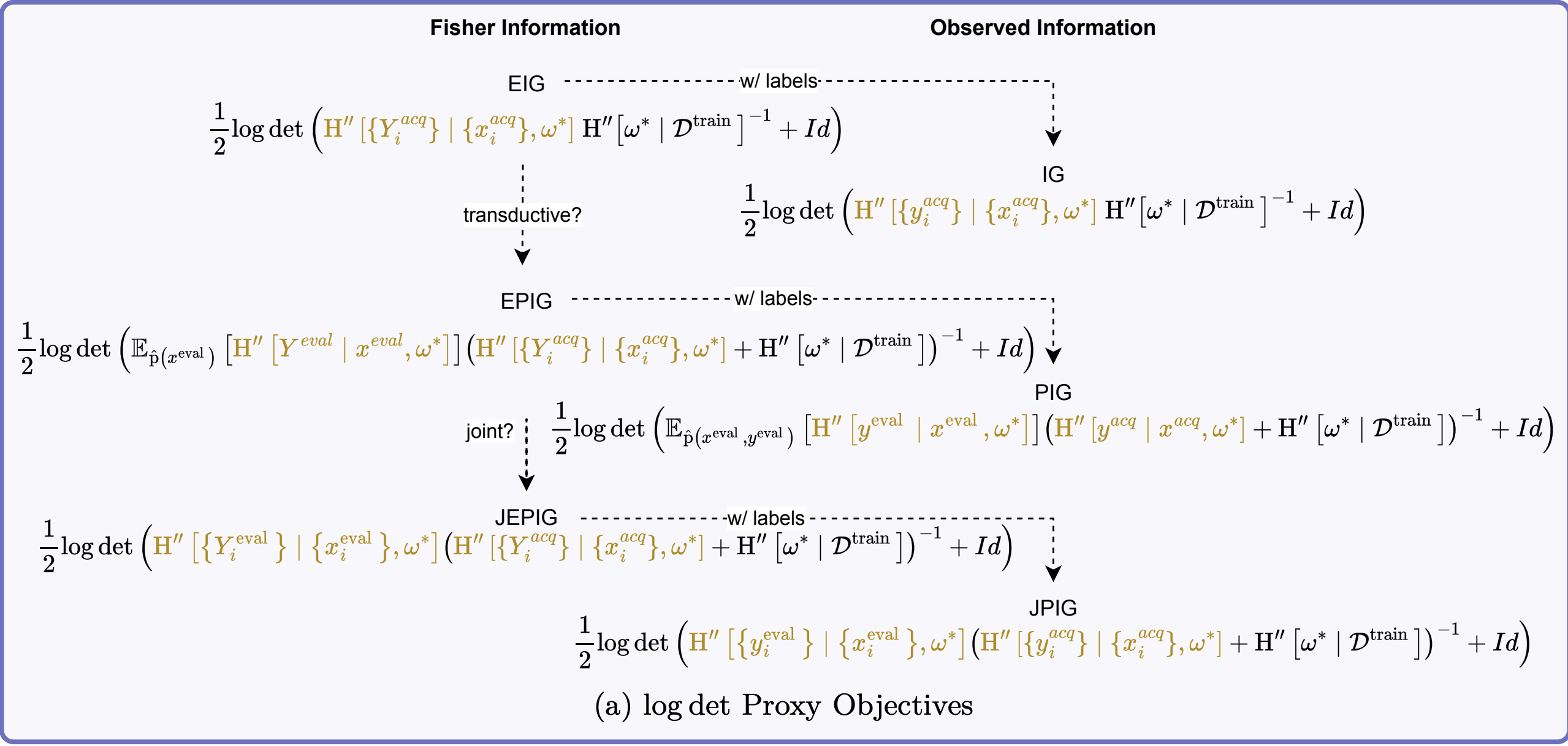
Key Information-Theoretic Objectives
Expected Information Gain (EIG): \[ \MIof{\W; \Y \given \x} = \Hof{\W} - \E{\pof{\y \given \x}}{\Hof{\W \given \y, \x}} \]
Information Gain (IG): Same as EIG but with known \(\yacq\) (for AS)
Expected Predictive Information Gain (EPIG): \[ \MIof{\Yeval; \Yacq \given \Xeval, \xacq} \]
Joint Expected Predictive Information Gain (JEPIG): \[ \MIof{\Yevalset; \Yacq \given \xevalset, \xacq} \]
Difference between EIG and JEPIG?
Expectation over \(\Yeval \given \xeval\) vs joint \(\Yevalset \given \xevalset\).
See also Hübotter et al. (2024) for a more detailed treatment of transductive active learning.
Part I: From Linear Regression to Fisher Information
Bayesian Linear Regression: A Worked Example
Model: \(y = \x^T \w + \epsilon\), where \(\epsilon \sim \mathcal{N}(0, \sigma_n^2)\)
Current posterior (dropped the \(\D\)): \(\pof{\w} = \mathcal{N}(\w | \mu, \Sigma_{old})\)
Posterior uncertainty: \(\Hof{\W} = \frac{1}{2} \log \det(2\pi e \Sigma_{old})\)
Goal: Select \(\xacq\) maximizing EIG
Key Insight: Posterior Update
After observing \((\xacq, \yacq)\):
\[ \Sigma_{new}^{-1} = \Sigma_{old}^{-1} + \frac{1}{\sigma_n^2} \xacq (\xacq)^T \]
Crucial: \(\Sigma_{new}\) does not depend on the observed value \(\yacq\)!
EIG for Linear Regression
\[ \begin{aligned} \text{EIG}(\xacq) &= \Hof{\W} - \E{\pof{\Yacq \given \xacq}}{\Hof{\W \given \Yacq, \xacq}} \\ &= \frac{1}{2} \log \det(\Sigma_{old} \Sigma_{new}^{-1}) \\ &= \frac{1}{2} \log \det\left(\Sigma_{old} \left(\Sigma_{old}^{-1} + \frac{1}{\sigma_n^2} \xacq (\xacq)^T\right)\right) \\ &= \frac{1}{2} \log \det\left(I_D + \frac{1}{\sigma_n^2} \Sigma_{old} \xacq (\xacq)^T\right) \end{aligned} \]
Using Sylvester’s Determinant Identity
\[ \det(I_M + AB) = \det(I_N + BA) \]
\[ \begin{aligned} \text{EIG}(\xacq) &= \frac{1}{2} \log \left(1 + \frac{(\xacq)^T \Sigma_{old} \xacq}{\sigma_n^2}\right) \end{aligned} \]
\[ \begin{aligned} \phantom{\text{EIG}(\xacq)}&= \frac{1}{2} \log \left(\frac{\sigma_n^2 + (\xacq)^T \Sigma_{old} \xacq}{\sigma_n^2}\right) \end{aligned} \]
The term \(\sigma_n^2 + (\xacq)^T \Sigma_{old} \xacq\) is the prior variance and \(\sigma_n^2\) is the posterior variance! This is just EIG = BALD.
Part II: Gaussian Approximations and Fisher Information
The Laplace Approximation
For general posteriors, approximate with a Gaussian:
\[ \w \overset{\approx}{\sim} \mathcal{N}(\wstar + ..., \HofHessian{\wstar}^{-1}) \]
where \(\HofHessian{\wstar} = -\nabla^2_\w \log \pof{\w\given\D}\) is the Hessian of negative log-posterior
Bayes’ rule for Hessians:
\[ \HofHessian{\w \given \D} = \HofHessian{\D \given \w} + \HofHessian{\w} \]
Bayes’ Rule and Additivity
For parameter inference with Bayes’ rule:
\[ \pof{\w\given\D} = \frac{\pof{\D\given\w}\pof{\w}}{\pof{\D}} \]
Taking the negative log and differentiating twice:
\[ \begin{aligned} \HofHessian{\w \given \D} &= -\nabla^2_\w \log \pof{\w\given\D} \\ &= -\nabla^2_\w \log \pof{\D\given\w} - \nabla^2_\w \log \pof{\w} \\ &= \HofHessian{\D \given \w} + \HofHessian{\w} \end{aligned} \]
This shows that Hessians are additive across independent data points (for the same \(\w\)):
\[ \HofHessian{\D \given \w} = \sum_{i=1}^N \HofHessian{y_i \given \w, \x_i} \]
Observed Information
The observed information is the Hessian of the negative log-likelihood for a specific observation:
\[ \HofHessian{y \given \x, \w } = -\nabla^2_\w \log \pof{y \given \x, \w} \]
While the Fisher Information Matrix (FIM) is the expected Hessian:
\[ \FisherInfo{Y \given \x, \w} = \E{\pof{y \given \x, \w}}{\HofHessian{y \given \x, \w}} \]
Fisher Information Matrix
The FIM is the expected Hessian of the negative log-likelihood:
\[\FisherInfo{Y \given \x, \w} = \E{\pof{y \given \x, \w}}{ \HofHessian{y \given \x, \w}}\]
The FIM has these important properties:
\[ \begin{aligned} \FisherInfo{Y \given \x, \w} &= \E{\pof{Y \given \x, \w}}{\HofJacobian{y \given \x, \w}^T \HofJacobian{y \given \x, \w}} \\ &= \implicitCov{\HofJacobian{Y \given \x, \w}^T} \\ &\succeq 0 \quad \text{(always positive semi-definite)} \end{aligned} \]
Exponential Family Distributions
For exponential family distributions
\[ \log \pof{y \given \prelogits} = \prelogits^T T(y) - A(\prelogits) + \log h(y) \]
with parameters \(\prelogits = f(x;\w)\), we have:
\[\FisherInfo{Y \given x, \w} = \nabla_\w f(x; \w)^T \, \nabla_\prelogits^2 A(\prelogits) \, \nabla_\w f(x; \w)\]
No expectation over \(y\) needed!
Examples:
- Normal distribution \(\pof{y \given \prelogits} = \mathcal{N}(y|\prelogits,1)\), \(\nabla_\prelogits^2 A(\prelogits) = 1\): \[\FisherInfo{Y \given x, \w} = \nabla_\w f(x; \w)^T \nabla_\w f(x; \w)\]
- Categorical distribution \(\pof{y \given \prelogits} = \text{softmax}(\prelogits)_y\), \(\nabla_\prelogits^2 A(\prelogits) = \text{diag}(\pi) - \pi\pi^T\): \[\FisherInfo{Y \given x, \w} = \nabla_\w f(x; \w)^T (\text{diag}(\pi) - \pi\pi^T) \nabla_\w f(x; \w)\]
Special Case: Generalized Linear Models
For GLMs (exponential family + linear mapping \(f(x;\w) = \w^T x\)):
\[\FisherInfo{Y \given x, \wstar} = \HofHessian{y \given x, \wstar} \quad \text{for any } y\]
Implication: Active learning and active sampling objectives coincide!
Generalized Gauss-Newton (GGN) Approximation
When we have an exponential family but not a GLM (e.g., deep neural networks), we often approximate the Hessian of the negative log-likelihood with the FIM: \[ \HofHessian{y \given x, \wstar} \approx \FisherInfo{Y \given x, \wstar} \] This GGN approximation is useful because the FIM is always positive semi-definite and can be more stable to compute.
Part III: Approximating Information Quantities
EIG Approximation via FIM
Starting from our Gaussian approximation: \[ \begin{aligned} \MIof{\W; \Yacq \given \xacq} &\approx \tfrac{1}{2}\E{}{\log \det \left(\HofHessian{\Yacq \given \xacq, \wstar}\HofHessian{\wstar}^{-1} + I\right)} \\ \end{aligned} \]
Connection to Bayesian Linear Regression
Recall EIG for BLR: \(\frac{1}{2} \log \left(1 + \frac{(\xacq)^T \Sigma_{old} \xacq}{\sigma_n^2}\right)\).
If \(\HofHessian{\wstar}^{-1} = \Sigma_{old}\) and \(\FisherInfo{\Yacq \given \xacq, \wstar} = \frac{1}{\sigma_n^2}\xacq (\xacq)^T\) (which holds for BLR), the approximation becomes exact.
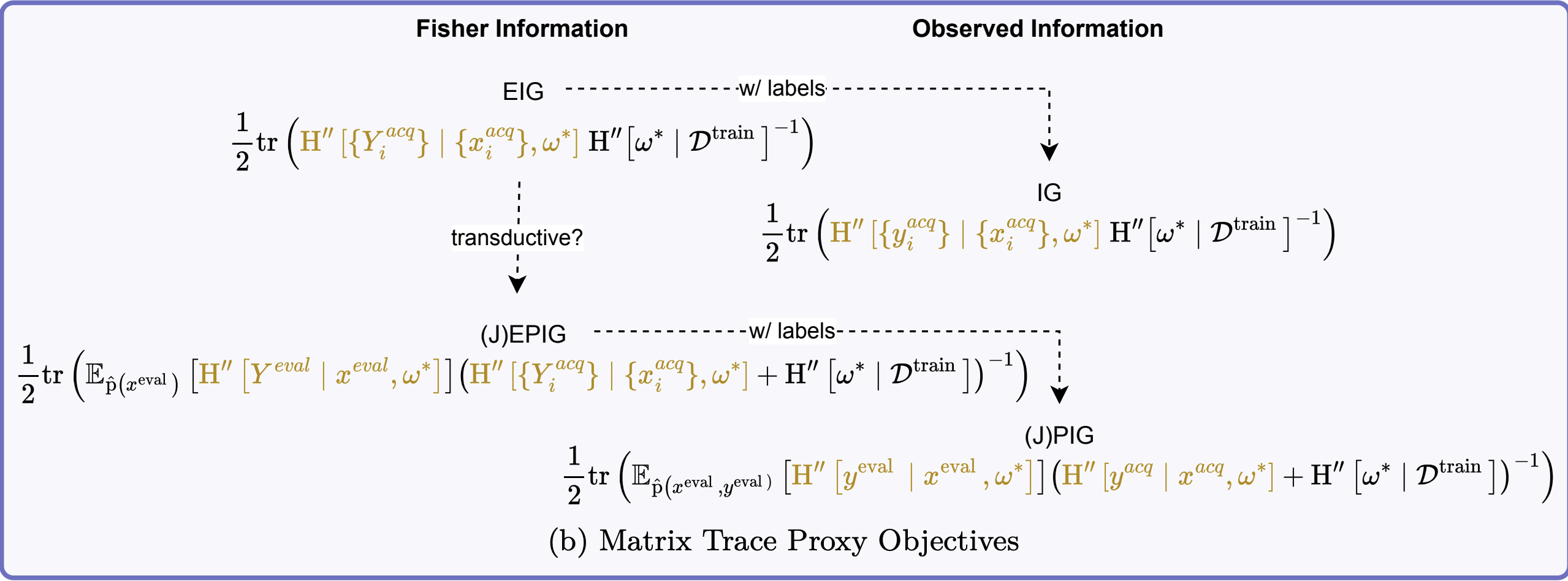
Trace Approximation
For computational efficiency, we can approximate using the trace:
\[ \log\det(I + A) \leq \tr(A) \]
This inequality holds for any positive semi-definite matrix \(A\). Applying this to our EIG approximation:
\[ \MIof{\W; \Yacq \given \xacq} \leq \tfrac{1}{2}\tr\left(\FisherInfo{\Yacq \given \xacq, \wstar}\HofHessian{\wstar}^{-1}\right) \]
The trace approximation only gives an upper bound but is easier to compute, especially for large models.
Batch Acquisition
The log-determinant form is not additive over acquisition samples: \[ \log \det\left(\sum_i \FisherInfo{\Yacq_i \given \xacq_i, \wstar}\HofHessian{\wstar}^{-1} + I\right) \]
The trace approximation is additive: \[ \sum_i \tr\left(\FisherInfo{\Yacq_i \given \xacq_i, \wstar}\HofHessian{\wstar}^{-1}\right) \]
Important
This means trace approximation ignores redundancies between batch samples (same issue as “top-k” BALD).
EPIG Approximation
Maximizing EPIG \(\MIof{\Yeval; \Yacq \given \Xeval, \xacq}\) is equivalent to minimizing the conditional mutual information \(\MIof{\W; \Yeval \given \Xeval, \Yacq, \xacq}\).
This is the EIG towards \(\Yeval \given \Xeval\) for the posteriors \(\pof{\w \given \Yacq, \xacq}\):
\[ \begin{aligned} &\MIof{\Yeval; \Yacq \given \Xeval, \xacq} \\ &\leq \tfrac{1}{2}\log \det\left(\opExpectation_{\pdataof{\xeval}} \left [ \FisherInfo{\Yeval \given \xeval, \wstar}\right ] \right. \\ &\quad \quad \left. (\FisherInfo{\Yacq \given \xacq, \wstar} + \HofHessian{\wstar})^{-1} + I\right) \end{aligned} \]
This is the actual foundation of BAIT (Ash et al., 2021)
Summary
Part IV: Similarity Matrices as FIM Approximations
From Gradients to FIM
Many methods use gradient similarity: \[ \similarityMatrix{}{\D \given \w}_{ij} = \langle \HofJacobian{y_i \given x_i, \wstar}, \HofJacobian{y_j \given x_j, \wstar} \rangle \]
Key insight: If we organize gradients into matrix \(\HofJacobianData{\D \given \wstar}\):
\[ \HofJacobianData{\D \given \wstar} = \begin{pmatrix} \vdots \\ \HofJacobian{y_i \given x_i, \wstar} \\ \vdots \end{pmatrix} \]
\[ \HofJacobianData{\D \given \wstar} = \begin{pmatrix} \vdots \\ \HofJacobian{y_i \given x_i, \wstar} \\ \vdots \end{pmatrix} \]
Then we get two complementary objects:
- \(\HofJacobianData{\D \given \wstar} \HofJacobianData{\D \given \wstar}^T\) yields the similarity matrix
- \(\HofJacobianData{\D \given \wstar}^T \HofJacobianData{\D \given \wstar}\) gives a one-sample estimate of the FIM
\[ \HofJacobianData{\D \given \wstar}^T \HofJacobianData{\D \given \wstar} \approx \FisherInfo{\Yset \given \xset, \wstar} \]
This is a one-sample Monte Carlo estimate of the FIM.
Caveats: Relies on (often hard) pseudo-labels for \(\y_i\), leading to a high-variance estimates of the true FIM (which expects over \(\pof{y \given x, \w}\)).
Similarity Matrix Form of EIG
With an uninformative prior (\(\HofHessian{\wstar} = \lambda I\) as \(\lambda \to 0\)), and using the Matrix Determinant Lemma, the EIG approximation can be written as:
\[ \MIof{\W; \Yacqset \given \xacqset} \approx \tfrac{1}{2}\log\det(\similarityMatrix{}{\Dacq \given \wstar}) \]
This is exactly what BADGE and SIMILAR optimize!
Part V: Unifying Popular Methods
BADGE (Ash et al., 2020)
- Uses k-means++ on gradient embeddings
- k-means++ approximately optimizes log-determinant
- Revealed: Approximating EIG with uninformative prior
BAIT (Ash et al., 2021)
- Directly implements trace approximation of EPIG. The objective maximized is: \[ \alpha(\xacqset) = \tr \left( \FisherInfo{\Yevalset \given \xevalset, \wstar} (\FisherInfo{\Yacqset \given \xacqset, \wstar} + \HofHessian{\wstar})^{-1} \right) \] where \(\HofHessian{\wstar}\) is the precision of the current posterior (e.g., from already labeled data \(\D_{train}\) and prior: \(\FisherInfo{\Ytrain \given \xtrain, \wstar} + \lambda I\)).
- Uses last-layer Fisher information
- Revealed: Principled transductive active learning
PRISM/SIMILAR
- LogDet objective: \(\log\det(\similarityMatrix{}{\Dacq \given \wstar})\)
- Revealed: Another EIG approximation
- LogDetMI variant approximates JEPIG
For transductive objectives (LogDetMI): \[ \begin{aligned} &\log \det \similarityMatrix{}{\Dacq \given \wstar} \\ &\quad - \log \det \left(\similarityMatrix{}{\Dacq \given \wstar} - \similarityMatrix{}{\Dacq ; \Deval \given \wstar} \right. \\ &\quad \quad \quad \left. \similarityMatrix{}{\Deval \given \wstar}^{-1} \similarityMatrix{}{\Deval ; \Dacq \given \wstar}\right) \end{aligned} \]
This approximates JEPIG!
Gradient Norm Methods (EGL, GraNd)
- Use \(\|\nabla_\w \mathcal{L}\|^2\)
- Revealed: Diagonal FIM approximation
- Trace of one-sample FIM estimate
Practical Takeaways
- When you see gradient-based AL methods, think “FIM approximation”
- LogDet objectives often work best because they approximate proper information quantities
- Trace approximations = dangerous for batch acquisition
- Last-layer approaches work well with pre-trained models
The Unification
- BADGE \(\approx\) EIG with uninformative prior
- BAIT \(\approx\) EPIG with trace approximation
- PRISM/SIMILAR (LogDet) \(\approx\) EIG/EPIG
- EGL/GraNd \(\approx\) EIG/IG with diagonal approximation
All are approximating the same few information-theoretic quantities!
What This Means
- Conceptual clarity: Seemingly different methods target the same objectives
- Cross-pollination: Improvements in one method may transfer to others
- Principled analysis: We can now understand why methods work or fail
Example: Trace approximations ignore batch redundancies → pathologies
Part VI: Insights and Implications
Weight vs Prediction Space
- Weight space (BADGE, BAIT, etc.):
- ✓ Computationally efficient
- ✗ Gaussian approximation quality
- ✗ May break in low-data regimes
- Prediction space (BALD, BatchBALD):
- ✓ More accurate information estimates
- ✗ Combinatorial explosion for batches
- ✗ Requires multiple model samples
Empirical Validation
- MNIST at 80 random samples
- Batch active learning for regression
MNIST at 80 Random Samples
High rank correlation between methods:
- BALD vs EIG (LogDet): ~0.95
- EPIG (Prediction) vs EPIG (LogDet): ~0.92
Weight-space methods preserve relative ranking!
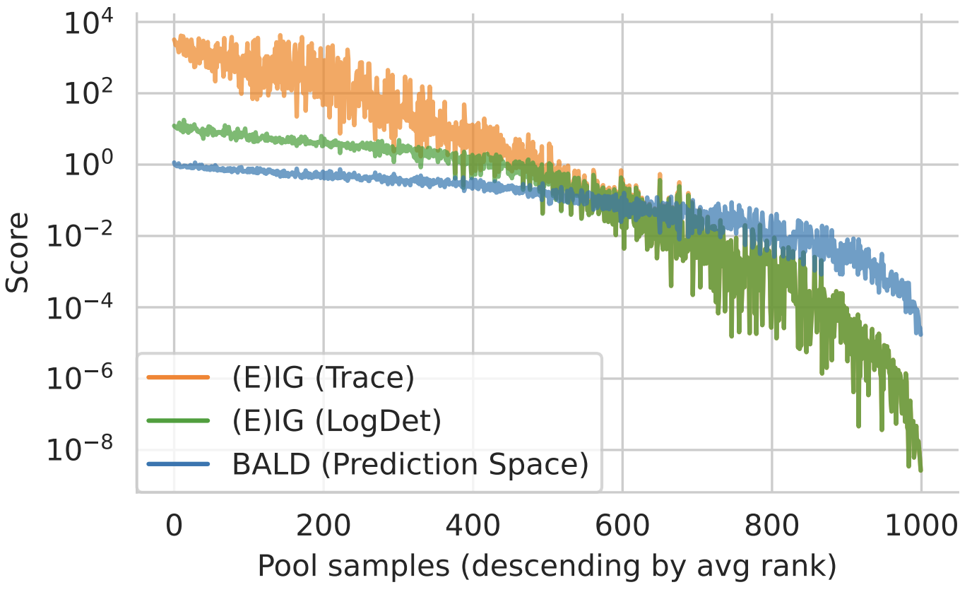
Figure 2: EIG Approximations. Trace and log det approximations match for small scores. They diverge for large scores. Qualitatively, the order matches the prediction-space approximation using BALD with MC dropout.
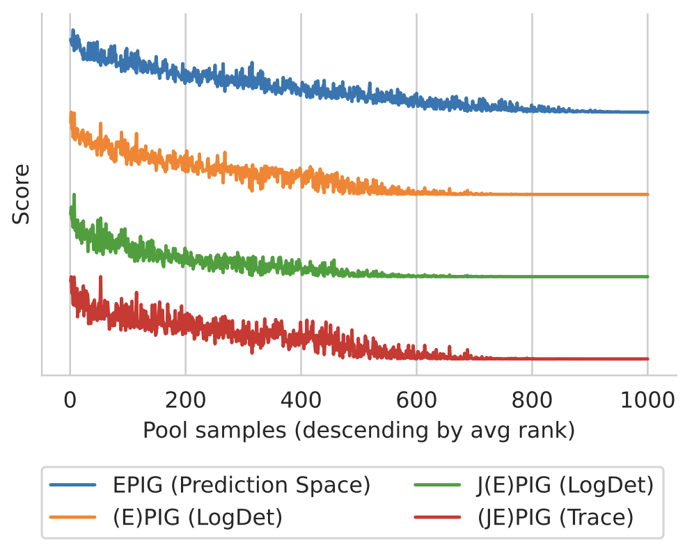
Figure 3: (J)EPIG Approximations (Normalized). The scores match qualitatively. Note we have reversed the ordering for the proxy objectives for JEPIG and EPIG as they are minimized while EPIG is maximized.
Black-box Batch Active Learning for Regression
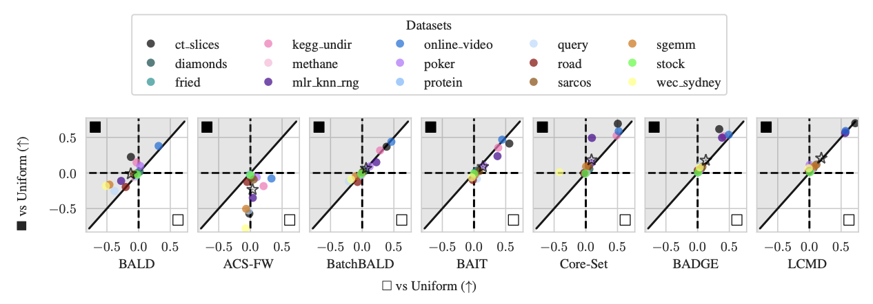
Figure 4: Average Logarithmic RMSE by regression datasets for DNNs: Black-box/prediction-space ■ vs white-box/weight-space □ (vs Uniform). Improvement of the white-box □ method over the uniform baseline on the x-axis and the improvement of the black-box ■ method over the uniform baseline on the y-axis. The average over all datasets is marked with a star ⋆.
Key Takeaways
Unification: Diverse methods optimize similar information-theoretic objectives
FIM as computational tool: Enables efficient approximation of complex quantities
Theory guides practice: Understanding connections helps design better algorithms
The Bigger Picture
Important
The “informativeness” that various methods try to capture collapses to the same information-theoretic quantities known since Lindley (1956) and MacKay (1992).
Understanding these connections allows us to build better, more principled active learning methods.
Future Directions
FIM approximations:
- Beyond pseudo-labels (expectations over predictive distributions)
- Multi-sample estimates (ensembles)
- Full-network approximations beyond last-layer
Batch selection: Using log-determinant approaches
Empirical validation: When do approximations break down in practice?
Thank You
Questions?
References
- Ash et al. (2020). Deep Batch Active Learning by Diverse, Uncertain Gradient Lower Bounds. ICLR.
- Ash et al. (2021). Gone Fishing: Neural Active Learning with Fisher Embeddings. NeurIPS.
- Holzmüller, D., Zaverkin, V., Kästner, J., & Steinwart, I. (2023). A framework and benchmark for deep batch active learning for regression. JMLR.
- Hübotter, J., Treven, L., As, Y., & Krause, A. (2024). Transductive active learning: Theory and applications. NeurIPS..
- Kirsch, Andreas (2023). “Black-box batch active learning for regression.” TMLR.
- Kothawade, S., Beck, N., Killamsetty, K., & Iyer, R. (2021). Similar: Submodular information measures based active learning in realistic scenarios. NeurIPS.