A Unifying Lens for Active Data Selection

Via the Fisher Information (Kirsch and Gal 2022)

1. Active learning methods have proliferated in recent years

2. The Fisher Information Matrix (FIM) provides a unifying lens

3. Many approaches approximate the same information-theoretic goals

4. This reveals key assumptions and future research directions

Empowerment Promise

\[ \require{mathtools} \DeclareMathOperator{\opExpectation}{\mathbb{E}} \newcommand{\E}[2]{\opExpectation_{#1} \left [ #2 \right ]} \newcommand{\simpleE}[1]{\opExpectation_{#1}} \newcommand{\implicitE}[1]{\opExpectation \left [ #1 \right ]} \DeclareMathOperator{\opVar}{\mathrm{Var}} \newcommand{\Var}[2]{\opVar_{#1} \left [ #2 \right ]} \newcommand{\implicitVar}[1]{\opVar \left [ #1 \right ]} \newcommand\MidSymbol[1][]{% \:#1\:} \newcommand{\given}{\MidSymbol[\vert]} \DeclareMathOperator{\opmus}{\mu^*} \newcommand{\IMof}[1]{\opmus[#1]} \DeclareMathOperator{\opInformationContent}{H} \newcommand{\ICof}[1]{\opInformationContent[#1]} \newcommand{\xICof}[1]{\opInformationContent(#1)} \newcommand{\sicof}[1]{h(#1)} \DeclareMathOperator{\opEntropy}{H} \newcommand{\Hof}[1]{\opEntropy[#1]} \newcommand{\xHof}[1]{\opEntropy(#1)} \DeclareMathOperator{\opMI}{I} \newcommand{\MIof}[1]{\opMI[#1]} \DeclareMathOperator{\opTC}{TC} \newcommand{\TCof}[1]{\opTC[#1]} \newcommand{\CrossEntropy}[2]{\opEntropy(#1 \MidSymbol[\Vert] #2)} \DeclareMathOperator{\opKale}{D_\mathrm{KL}} \newcommand{\Kale}[2]{\opKale(#1 \MidSymbol[\Vert] #2)} \DeclareMathOperator{\opJSD}{D_\mathrm{JSD}} \newcommand{\JSD}[2]{\opJSD(#1 \MidSymbol[\Vert] #2)} \DeclareMathOperator{\opp}{p} \newcommand{\pof}[1]{\opp(#1)} \newcommand{\pcof}[2]{\opp_{#1}(#2)} \newcommand{\hpcof}[2]{\hat{\opp}_{#1}(#2)} \DeclareMathOperator{\opq}{q} \newcommand{\qof}[1]{\opq(#1)} \newcommand{\qcof}[2]{\opq_{#1}(#2)} \newcommand{\varHof}[2]{\opEntropy_{#1}[#2]} \newcommand{\xvarHof}[2]{\opEntropy_{#1}(#2)} \newcommand{\varMIof}[2]{\opMI_{#1}[#2]} \newcommand{\Y}{Y} \newcommand{\y}{y} \newcommand{\X}{\boldsymbol{X}} \newcommand{\x}{\boldsymbol{x}} \newcommand{\w}{\boldsymbol{\theta}} \newcommand{\wstar}{\boldsymbol{\theta^*}} \newcommand{\W}{\boldsymbol{\Theta}} \newcommand{\D}{\mathcal{D}} \DeclareMathOperator{\opf}{f} \newcommand{\fof}[1]{\opf(#1)} \newcommand{\indep}{\perp\!\!\!\!\perp} \newcommand{\HofHessian}[1]{\opEntropy''[#1]} \newcommand{\specialHofHessian}[2]{\opEntropy''_{#1}[#2]} \newcommand{\HofJacobian}[1]{\opEntropy'[#1]} \newcommand{\specialHofJacobian}[2]{\opEntropy'_{#1}[#2]} \DeclareMathOperator{\tr}{tr} \DeclareMathOperator{\opCovariance}{\mathrm{Cov}} \newcommand{\Cov}[2]{\opCovariance_{#1} \left [ #2 \right ]} \newcommand{\implicitCov}[1]{\opCovariance \left [ #1 \right ]} \newcommand{\FisherInfo}{\HofHessian} \newcommand{\prelogits}{\boldsymbol{z}} \newcommand{\typeeval}{\mathrm{eval}} \newcommand{\typetest}{\mathrm{test}} \newcommand{\typetrain}{\mathrm{train}} \newcommand{\typeacq}{\mathrm{acq}} \newcommand{\typepool}{\mathrm{pool}} \newcommand{\xeval}{\x^\typeeval} \newcommand{\xtest}{\x^\typetest} \newcommand{\xtrain}{\x^\typetrain} \newcommand{\xacq}{\x^\typeacq} \newcommand{\xpool}{\x^\typepool} \newcommand{\xacqsettar}{\x^{\typeacq, *}} \newcommand{\Xeval}{\X^\typeeval} \newcommand{\Xtest}{\X^\typetest} \newcommand{\Xtrain}{\X^\typetrain} \newcommand{\Xacq}{\X^\typeacq} \newcommand{\Xpool}{\X^\typepool} \newcommand{\yeval}{\y^\typeeval} \newcommand{\ytest}{\y^\typetest} \newcommand{\ytrain}{\y^\typetrain} \newcommand{\yacq}{\y^\typeacq} \newcommand{\ypool}{\y^\typepool} \newcommand{\Ytest}{\Y^\typetest} \newcommand{\Ytrain}{\Y^\typetrain} \newcommand{\Yeval}{\Y^\typeeval} \newcommand{\Yacq}{\Y^\typeacq} \newcommand{\Ypool}{\Y^\typepool} \newcommand{\Xrate}{\boldsymbol{\mathcal{\X}}} \newcommand{\Yrate}{\mathcal{\Y}} \newcommand{\batchvar}{\mathtt{K}} \newcommand{\poolsize}{\mathtt{M}} \newcommand{\trainsize}{\mathtt{N}} \newcommand{\evalsize}{\mathtt{E}} \newcommand{\testsize}{\mathtt{T}} \newcommand{\numclasses}{\mathtt{C}} \newcommand{\xevalset}{{\x^\typeeval_{1..\evalsize}}} \newcommand{\xtestset}{{\x^\typetest_{1..\testsize}}} \newcommand{\xtrainset}{{\x^\typetrain_{1..\trainsize}}} \newcommand{\xacqset}{{\x^\typeacq_{1..\batchvar}}} \newcommand{\xpoolset}{{\x^\typepool_{1..\poolsize}}} \newcommand{\xacqsetstar}{{\x^{\typeacq, *}_{1..\batchvar}}} \newcommand{\Xevalset}{{\X^\typeeval_{1..\evalsize}}} \newcommand{\Xtestset}{{\X^\typetest_{1..\testsize}}} \newcommand{\Xtrainset}{{\X^\typetrain_{1..\trainsize}}} \newcommand{\Xacqset}{{\X^\typeacq_{1..\batchvar}}} \newcommand{\Xpoolset}{{\X^\typepool_{1..\poolsize}}} \newcommand{\yevalset}{{\y^\typeeval_{1..\evalsize}}} \newcommand{\ytestset}{{\y^\typetest_{1..\testsize}}} \newcommand{\ytrainset}{{\y^\typetrain_{1..\trainsize}}} \newcommand{\yacqset}{{\y^\typeacq_{1..\batchvar}}} \newcommand{\ypoolset}{{\y^\typepool_{1..\poolsize}}} \newcommand{\Ytestset}{{\Y^\typetest_{1..\testsize}}} \newcommand{\Ytrainset}{{\Y^\typetrain_{1..\trainsize}}} \newcommand{\Yevalset}{{\Y^\typeeval_{1..\evalsize}}} \newcommand{\Yacqset}{{\Y^\typeacq_{1..\batchvar}}} \newcommand{\Ypoolset}{{\Y^\typepool_{1..\poolsize}}} \newcommand{\yset}{{\y_{1..n}}} \newcommand{\Yset}{{\Y_{1..n}}} \newcommand{\xset}{{\x_{1..n}}} \newcommand{\Xset}{{\X_{1..n}}} \newcommand{\pdataof}[1]{\hpcof{\mathrm{true}}{#1}} \newcommand{\ptrainof}[1]{\hpcof{\mathrm{train}}{#1}} \newcommand{\similarityMatrix}[2]{{S_{#1}[#2]}} \newcommand{\HofJacobianData}[1]{{\hat{\opEntropy}'[#1]}} \newcommand{\HofJacobianDataShort}{\hat{\opEntropy}'} \newcommand{\Dacq}{\D^{\typeacq}} \newcommand{\Dtest}{\D^{\typetest}} \newcommand{\Dpool}{\D^{\typepool}} \newcommand{\Deval}{\D^{\typeeval}} \]

By lecture’s end, when you see methods like BADGE, BAIT, or PRISM, you’ll immediately recognize:

• “Ah, BADGE is approximating EIG with an uninformative prior!”
• “BAIT is using a trace approximation of EPIG”
• “These gradient similarity matrices are just one-sample FIM estimates!”

You’ll move from memorizing formulas to understanding the deeper structure.

I. Background

A. Active Data Selection

• Active Learning (AL): Which unlabeled data point, if labeled, would be most informative for model training?
  • Goal: Label efficiency.
• Active Sampling (AS): Which labeled data point from a large training set is most informative to train on next?
  • Goal: Training efficiency, coreset selection, curriculum learning.
• The common thread: Quantifying “informativeness.”

B. Acquisition Functions

1. Expected Information Gain (EIG / BALD):
   • \(\begin{aligned} &\MIof{\W; \Yacq \given \x^{acq}} = \Hof{\W} - \Hof{\W \given \Yacq, \x^{acq}} \\ &\quad = \Hof{\W} - \E{\pof{\yacq \given \x^{acq}}}{\Hof{\W \given \yacq, \x^{acq}}} \end{aligned}\)
   • Measures reduction in model parameter uncertainty.
   • Key idea: Select data that maximally reduces what we don’t know about the model.

2. Information Gain (IG):
   • \(\MIof{\W; \yacq \given \x^{acq}} = \Hof{\W} - \Hof{\W \given \yacq, \x^{acq}}\)
   • Similar to EIG, but \(\yacq\) is known (for AS).

3. Expected Predictive Information Gain (EPIG): \(\MIof{\Yeval; \Yacq \given \Xeval, \x^{acq}}\)
   • Measures information gain about other unseen data points.
   • Transductive: Considers impact on a specific evaluation/pool set.
4. Joint Expected Predictive Information Gain (JEPIG): \(\MIof{\Yevalset; \Yacq \given \xevalset, \x^{acq}}\)
   • Transductive: Considers impact on a specific evaluation/pool set.

These are often hard to compute directly for complex models.

II. Example: Bayesian Linear Regression

A. Setup

• Model: Consider a linear model: \(y = \x^T \w + \epsilon\), where \(\epsilon \sim \mathcal{N}(0, \sigma_n^2)\) is Gaussian noise with known variance \(\sigma_n^2.\) The parameters are \(\w \in \mathbb{R}^D\).

• Bayesian Inference: The current posterior, based on observed data \(\D\) (which we drop for simplicity):

  \[ \pof{\w} = \mathcal{N}(\w | \mu, \Sigma) \]

• Goal: Select unlabeled data point \(\x^{acq}\) maximizing: \[ \text{EIG}(\x^{acq}) = \Hof{\W} - \E{\pof{\yacq \given \x^{acq}}}{\Hof{\W \given \yacq, \x^{acq}}} \]

Slide 1: Bayesian Linear Regression: Model & EIG Goal

• Entropy of a Gaussian Distribution: For a multivariate Gaussian \(\pof{\W} = \mathcal{N}(\boldsymbol{\mu}, \boldsymbol{\Sigma})\), the differential entropy is \(\Hof{\W} = \frac{1}{2} \log \det(2\pi e \boldsymbol{\Sigma})\).

• Current Parameter Entropy: The entropy of our current posterior \(\pof{\W}\) is:

  \[ \Hof{\W} = \frac{1}{2} \log \det(2\pi e \Sigma) \]

Slide 2: Bayesian Linear Regression: EIG Derivation

B. Observing \((\x^{acq}, \yacq)\)

If we observe \(\yacq\) for \(\x^{acq}\), the new posterior \(\pof{\w \given \yacq, \x^{acq}}\) is also Gaussian \(\mathcal{N}(\w | \mu_{new}, \Sigma_{new})\) with:

\[ \Sigma_{new}^{-1} = \Sigma^{-1} + \frac{1}{\sigma_n^2} \x^{acq} (\x^{acq})^T \]

Important

This updated covariance \(\Sigma_{new}\) does not depend on the observed value \(\yacq\). Only the mean \(\mu_{new}\) depends on \(\yacq\).

C. Expected Posterior Entropy

• The entropy of the parameters given \(\yacq\) and \(\x^{acq}\) is \[ \Hof{\W \given \Yacq, \x^{acq}} = \frac{1}{2} \log \det(2\pi e \Sigma_{new}) \]

• Since \(\Sigma_{new}\) (and thus this entropy term) does not depend on \(\yacq\), the expectation over \(p(\yacq | \x^{acq})\) is trivial:

  \[ \E{\pof{\yacq \given \x^{acq}}}{\Hof{\W \given \yacq, \x^{acq}}} = \frac{1}{2} \log \det(2\pi e \Sigma_{new}) \]

D. Putting it all together

\[ \begin{aligned} \text{EIG}(\x^{acq}) &= \Hof{\W} - \E{\pof{\Yacq \given \x^{acq}}}{\Hof{\W \given \Yacq, \x^{acq}}} \\ &= \frac{1}{2} \log \det(2\pi e \Sigma) - \frac{1}{2} \log \det(2\pi e \Sigma_{new}) \\ &= \frac{1}{2} \log \left( \frac{\det(\Sigma)}{\det(\Sigma_{new})} \right) = \frac{1}{2} \log \det(\Sigma \Sigma_{new}^{-1}) \end{aligned} \]

Substituting \(\Sigma_{new}^{-1} = \Sigma^{-1} + \frac{1}{\sigma_n^2} \x^{acq} (\x^{acq})^T\):

\[ \begin{aligned} \text{EIG}(\x^{acq}) &= \frac{1}{2} \log \det\left(\Sigma \left(\Sigma^{-1} + \frac{1}{\sigma_n^2} \x^{acq} (\x^{acq})^T\right)\right) \\ &= \frac{1}{2} \log \det\left(I_D + \frac{1}{\sigma_n^2} \Sigma \x^{acq} (\x^{acq})^T\right) \\ &\le \frac{1}{2} \tr \left( \Sigma \x^{acq} (\x^{acq})^T \right) \end{aligned} \] where \(I_D\) is the \(D \times D\) identity matrix.

E. Sylvester’s Determinant Identity

\[ \det(I_M + AB) = \det(I_N + BA) \]

\[ \begin{aligned} A &:= \frac{1}{\sigma_n^2} \Sigma \x^{acq} \text{ (a $D \times 1$ column vector) and } \\ B &:= (\x^{acq})^T \text{ (a $1 \times D$ row vector)} \\ BA &= \frac{1}{\sigma_n^2} (\x^{acq})^T \Sigma \x^{acq} \text{ (a scalar)} \end{aligned} \]

\[ \implies \text{EIG}(\x^{acq}) = \frac{1}{2} \log \left(1 + \frac{1}{\sigma_n^2} (\x^{acq})^T \Sigma \x^{acq}\right) \]

F. Interpretation

• The term \(v_f(\x^{acq}) = (\x^{acq})^T \Sigma \x^{acq}\) is the variance of the model’s prediction for the underlying function \(f(\x^{acq}) = (\x^{acq})^T\w\) under the current posterior \(\pof{\w}\). It reflects the model’s uncertainty about \(f(\x^{acq})\).

\[ \begin{aligned} \text{EIG}(\x^{acq}) &= \frac{1}{2} \log \left(1 + \frac{v_f(\x^{acq})}{\sigma_n^2}\right) \\ &= \frac{1}{2} \log \left(\frac{\sigma_n^2 + v_f(\x^{acq})}{\sigma_n^2}\right) \end{aligned} \]

G. BALD

\[ \begin{aligned} \text{EIG}(\x^{acq}) &= \frac{1}{2} \log \left(1 + \frac{v_f(\x^{acq})}{\sigma_n^2}\right) \\ &= \frac{1}{2} \log \left(\frac{\sigma_n^2 + v_f(\x^{acq})}{\sigma_n^2}\right) \\ &= \Hof{\Yacq \given \x^{acq}} - \Hof{\Yacq \given \x^{acq}, \W} \\ &= \MIof{\Yacq; \W \given \x^{acq}}. \end{aligned} \]

“\(\Leftrightarrow\) EIG = BALD (Bayesian Active Learning by Disagreement)” (Houlsby et al. 2011), \(\MIof{\Yacq; \W \given \x^{acq}}\), for this Gaussian model.

H. Summary

1. EIG measures a reduction in uncertainty given a candidate point.
2. Gaussian Entropies are \(\frac{1}{2} \log \det(2\pi e \boldsymbol{\Sigma})\).
3. \(\Sigma_{new}\) is independent of the label \(\yacq\).
4. Parameter EIG becomes \(\frac{1}{2} \log \det(\Sigma \Sigma_{new}^{-1})\).
5. \(\log \det(\Sigma + Id) \le \tr(\Sigma)\).
6. A determinant identity transforms from weight space to prediction space.

Next: Laplace as Gaussian approximation.

Let’s briefly recap the journey for our Bayesian Linear Regression example:

1. EIG Definition: We started with EIG as the reduction in parameter entropy: \(\text{EIG}(\x^{acq}) = \Hof{\W} - \E{\pof{\Yacq \given \x^{acq}}}{\Hof{\W \given \Yacq, \x^{acq}}}\).

2. Gaussian Entropies: For Gaussian posteriors, entropy is \(\frac{1}{2} \log \det(2\pi e \boldsymbol{\Sigma})\). The \(2\pi e\) terms cancel.

3. Key Simplification: The updated posterior covariance \(\Sigma_{new}\) (after observing \(\x^{acq}\)) was independent of the label \(\yacq\). This made the expectation trivial. \[ \Sigma_{new}^{-1} = \Sigma^{-1} + \frac{1}{\sigma_n^2} \x^{acq} (\x^{acq})^T \]

4. Log-Determinant Form: EIG became \(\frac{1}{2} \log \det(\Sigma \Sigma_{new}^{-1})\).

5. Sylvester’s Identity: Using \(\det(I + AB) = \det(I + BA)\), we transformed the expression: \[ \text{EIG}(\x^{acq}) = \frac{1}{2} \log \det\left(I_D + \frac{1}{\sigma_n^2} \Sigma \x^{acq} (\x^{acq})^T\right) \] \[ \implies \text{EIG}(\x^{acq}) = \frac{1}{2} \log \left(1 + \frac{1}{\sigma_n^2} (\x^{acq})^T \Sigma \x^{acq}\right) \]

6. Predictive Variance: The term \((\x^{acq})^T \Sigma \x^{acq}\) is the model’s predictive variance \(v_f(\x^{acq})\) for \(f(\x^{acq})\). \[ \text{EIG}(\x^{acq}) = \frac{1}{2} \log \left(1 + \frac{v_f(\x^{acq})}{\sigma_n^2}\right) \] This connects EIG directly to selecting points where the model is most uncertain about the underlying function.

III. Laplace Approximation \(\approx\) Gaussian Approximation

• Our goal: Approximate the posterior \(\pof{\w \given \D}\) using a Gaussian distribution
• Key insight: Use Taylor expansion of Shannon’s information content (negative log likelihood)
• Information content \(\Hof{\w} = -\log \pof{\w \given \D}\) (note lowercase \(\w\))

A. Deriving the Approximation

Using a second-order Taylor expansion around \(\wstar\):

\[ \begin{aligned} \Hof{\w} \approx \Hof{\wstar} &+ \nabla_{\w} \Hof{\wstar} (\w - \wstar) \\ &+ \frac{1}{2}(\w - \wstar)^T \nabla_{\w}^2 \Hof{\wstar} (\w - \wstar) \end{aligned} \]

Simplifying notation with \(\HofJacobian{\wstar} = \nabla_{\w} \Hof{\wstar}\) and \(\HofHessian{\wstar} = \nabla_{\w}^2 \Hof{\wstar}\):

\[ \begin{aligned} \Hof{\w} \approx \Hof{\wstar} &+ \HofJacobian{\wstar} (\w - \wstar) \\ &+ \frac{1}{2}(\w - \wstar)^T H''[\wstar] (\w - \wstar) \end{aligned} \]

B. Completing the Square

We can rewrite this by completing the square:

\[ \begin{aligned} \Hof{\w} &\approx \frac{1}{2}(\w - (\wstar - \HofHessian{\wstar}^{-1}\HofJacobian{\wstar})^T)^T H''[\wstar] \\ &\quad \quad (\w - (\wstar - \HofHessian{\wstar}^{-1}\HofJacobian{\wstar})^T) + \text{const.} \end{aligned} \]

This resembles the information content of a Gaussian distribution:

\[H(\mathcal{N}(\boldsymbol{\mu}, \boldsymbol{\Sigma})) = \frac{1}{2}(\w - \boldsymbol{\mu})^T \boldsymbol{\Sigma}^{-1} (\w - \boldsymbol{\mu}) + \text{const.}\]

C. The Gaussian Approximation

• This gives us the Gaussian approximation:

  \[ \w \overset{\approx}{\sim} \mathcal{N}(\wstar - \HofHessian{\wstar}^{-1}\HofJacobian{\wstar}^T, \HofHessian{\wstar}^{-1}) \]

• If \(\wstar\) is a (local) minimizer of \(\Hof{\w}\), then \(\HofJacobian{\wstar} = 0\), yielding the Laplace approximation:

  \[ \w \overset{\approx}{\sim} \mathcal{N}(\wstar, \HofHessian{\wstar}^{-1}) \]

D. Precision and Hessian Matrix

• For the Gaussian approximation, the Hessian matrix \(\HofHessian{\wstar}\) is the precision matrix (inverse covariance) of the approximate posterior:

  \[\Sigma^{-1} = \HofHessian{\wstar}\]

• Therefore, the entropy of our Gaussian approximation is:

  \[\Hof{\W} \approx -\frac{1}{2}\log\det\HofHessian{\wstar} + \frac{k}{2}\log(2\pi e)\]

  where \(k\) is the dimensionality of \(\w\).

• This approximation allows us to compute entropy differences by focusing on the change in the log-determinant of the Hessian.

• Note: The constant term \(\frac{k}{2}\log(2\pi e)\) cancels out when computing information quantities involving entropy differences (hint hint: mutual information).

E. Bayes’ Rule for Hessians

• When we apply Bayes’ rule to parameter inference:

  \[ \pof{\w\given\D} = \frac{\pof{\D\given\w}\pof{\w}}{\pof{\D}} \]

• Taking the negative log and differentiating twice:

  \[ \begin{aligned} \HofHessian{\w \given \D} &= -\nabla^2_\w \log \pof{\w\given\D} \\ &= -\nabla^2_\w \log \left[\frac{\pof{\D\given\w}\pof{\w}}{\pof{\D}}\right] \end{aligned} \]

• Using the additivity of logarithms:

  \[ \begin{aligned} \HofHessian{\w \given \D} &= -\nabla^2_\w \left[\log \pof{\D\given\w} + \log \pof{\w} - \log \pof{\D}\right] \end{aligned} \]

• Since \(\pof{\D}\) is constant with respect to \(\w\), its Hessian is zero:

  \[ \HofHessian{\w \given \D} = -\nabla^2_\w \log \pof{\D\given\w} - \nabla^2_\w \log \pof{\w} \]

• So we have the Hessian’s Bayes’ rule:

  \[ \HofHessian{\w \given \D} = \HofHessian{\D \given \w} + \HofHessian{\w} \]

\[ \HofHessian{\w \given \D} = \HofHessian{\D \given \w} + \HofHessian{\w} = \HofHessian{\w, \D} \]

In terms of precision matrices for our Gaussian approximation:

\[ \Sigma_{\text{posterior}}^{-1} = \Sigma_{\text{likelihood}}^{-1} + \Sigma_{\text{prior}}^{-1} \]

(when we treat the likelihood as unnormalized Gaussian)

F. Observed Information

\(\HofHessian{\D \given \w}\) is also called the observed information. It is the Hessian of the log-likelihood and also additive in the data points:

\[ \HofHessian{\D \given \w} = \sum_{i=1}^N \HofHessian{y_i \given \w, \x_i}. \]

G. Fisher Information Matrix

• The Fisher Information Matrix (FIM) is the expected Hessian of the log-likelihood:

  \[ \HofHessian{Y \given \x, \w }= \E{\pof{y \given \x, \w}}{ \HofHessian{y \given \x, \w}}. \]

• We have the following identities:

  \[ \begin{aligned} \HofHessian{Y \given \x, \w} &= \E{\pof{Y \given \x, \w}}{ \HofJacobian{y \given \x, \w}^T \HofJacobian{y \given \x, \w} } \\ &= \implicitCov{\HofJacobian{Y \given \x, \w}^T} \\ &\succeq 0 \quad \text{(positive semi-definite)} \end{aligned} \]

IV. Special Cases of Fisher Information

A. Exponential Family

• \(\Leftrightarrow\) \(\pof{y \given \prelogits=f(x;\w)}\) with \(f(x;\w)\) the logits and \(\pof{y \given \prelogits}\) from the exponential family:

  \[ \log \pof{y \given \prelogits} = \prelogits^T T(y) - A(\prelogits) + \log h(y) \]

• Fisher information becomes independent of \(y\):

  \[\FisherInfo{Y \given x, \w} = \nabla_\w f(x; \w)^T \, {\nabla_\prelogits^2 A(\prelogits) |_{\prelogits=f(x ; \w)}} \, \nabla_\w f(x; \w)\]

• This simplifies computation: no \(\opExpectation\) over \(y\) is needed!

B. Normal Distribution

• \(\Leftrightarrow\) \(\pof{y \given \prelogits} = \mathcal{N}(y|\prelogits,1)\)

• We have:

  • \(A(\prelogits) = \frac{\prelogits^2}{2}\)
  • \(\nabla_\prelogits^2 A(\prelogits) = 1\)

• The Fisher information simplifies to:

  \[\FisherInfo{Y \given x, \w} = \nabla_\w f(x; \w)^T \, \nabla_\w f(x; \w)\]

• This is simply the outer product of the gradients of the network outputs with respect to the parameters

C. Categorical Distribution

• \(\Leftrightarrow\) \(\pof{y \given \prelogits} = \text{softmax}(\prelogits)_y\)

• \(\nabla_\prelogits^2 A(\prelogits) = \text{diag}(\pi) - \pi\pi^T\), where \(\pi_y=\pof{y \given \prelogits}\)

• Thus:

  \[ \FisherInfo{Y \given x, \w} = \nabla_\w f(x; \w)^T \, (\text{diag}(\pi) - \pi\pi^T) \, \nabla_\w f(x; \w) \]

• This captures the geometry of parameter space for classification problems

D. Generalized Linear Models

• Definition: A GLM combines:

  1. An exponential family distribution for \(\pof{y \given \prelogits}\)
  2. A linear mapping for the logits: \(f(x;\w) = \w^T \x\)

• Key insight: Not only is Fisher information independent of \(y\) for a GLM, but the observed information is too!

  \[ \HofHessian{y \given x, \w} = \x^T \, \nabla_\prelogits^2 A(f(x; \w)) \, \x \]

E. The GLM Connection

• For GLMs, we have the remarkable equality:

  \[\FisherInfo{Y \given x, \wstar} = \HofHessian{y \given x, \wstar}\]

  for any \(y\) (the observed information is independent of \(y\))

• This means expectations over data distributions equal expectations over model distributions.

• Why this matters: We would often like an expectation over the true data distribution, but we only have the model’s predictive distribution!

F. Generalized Gauss-Newton Approximation

• When we have an exponential family but not a GLM, we often approximate:

  \[\HofHessian{y \given x, \wstar} \approx \FisherInfo{Y \given x, \wstar}\]

• This is the Generalized Gauss-Newton (GGN) approximation

G. Benefits of GGN

• Always positive semi-definite (unlike the true Hessian)
• Computationally more stable
• Connects active learning and active sampling objectives

H. Last-Layer Approach

• Treat only the last layer as parameters

• Write model as \(p(y|x,\w) = p(y|\prelogits = \w^T \phi(x))\), where:

  • \(\phi(x)\) is the embedding from lower layers (treated as fixed)
  • \(\w\) contains only the last-layer weights

• This creates a GLM on top of fixed embeddings

• The practical simplification while preserving many benefits?

• Used by BADGE, BAIT, PRISM, SIMILAR in practice

Key Takeaway

Important

The special structure of GLMs and exponential families bridges the gap between active learning (which doesn’t know labels) and active sampling (which does).

For these models, acquisition functions that seem different are actually optimizing the same objectives!

V. Approximating EIG and EPIG with Fisher Information

A. Approximating the EIG

Start with the EIG decomposition:

\[ \begin{aligned} \MIof{\W; \Yacq \given \xacq} &= \Hof{\W} - \Hof{\W \given \Yacq, \xacq} \\ &= \Hof{\W} - \E{\pof{\yacq \given \xacq}}{\Hof{\W \given \yacq, \xacq}} \end{aligned} \]

(I’ll drop the \(\pof{\yacq \given \xacq}\) from the expectation from now on.)

Applying the Gaussian approximation:

\[ \begin{aligned} &\approx -\tfrac{1}{2}\log \det \HofHessian{\wstar} - \E{}{-\tfrac{1}{2}\log \det \HofHessian{\wstar \given \Yacq, \xacq}} \\ &= \tfrac{1}{2}\E{}{\log \det \HofHessian{\wstar \given \Yacq, \xacq} \, \HofHessian{\wstar}^{-1}} \\ &= \tfrac{1}{2}\E{}{\log \det (\HofHessian{\Yacq \given \xacq, \wstar} + \HofHessian{\wstar}) \, \HofHessian{\wstar}^{-1}} \\ &= \tfrac{1}{2}\E{}{\log \det \left(\HofHessian{\Yacq \given \xacq, \wstar}\HofHessian{\wstar}^{-1} + I\right)} \end{aligned} \]

B. EIG for GLMs

For GLMs (or with GGN approximation), we can simplify further (for any \(\yacq\)):

\[ \begin{aligned} &\MIof{\W; \Yacq \given \xacq} \\ &\quad \approx \tfrac{1}{2}\log \det\left(\FisherInfo{\yacq \given \xacq, \wstar}\HofHessian{\wstar}^{-1} + I\right) \end{aligned} \]

We can also use the trace approximation:

\[ \begin{aligned} \MIof{\W; \Yacq \given \xacq} &\leq \tfrac{1}{2}\tr\left(\FisherInfo{\Yacq \given \xacq, \wstar}\HofHessian{\wstar}^{-1}\right) \end{aligned} \]

C. \(\leftrightarrow\) Bayesian Linear Regression

Remember our solution for Bayesian linear regression:

\[ \text{EIG}(\x^{acq}) = \frac{1}{2} \log \det\left(I_D + \Sigma \x^{acq} \frac{1}{\sigma_n^2} (\x^{acq})^T\right) \]

Compare to our general approximation:

\[ \approx \tfrac{1}{2}\log \det\left(\FisherInfo{\Yacq \given \xacq, \wstar}\HofHessian{\wstar}^{-1} + I\right) \]

For linear regression, our approximation is exact (of course)!

D. Batch Acquisition

• The log-determinant form is not additive over acquisition samples: \[ \log \det\left(\sum_i \FisherInfo{\Yacq_i \given \xacq_i, \wstar}\HofHessian{\wstar}^{-1} + I\right) \]

• The trace approximation is additive: \[ \sum_i \tr\left(\FisherInfo{\Yacq_i \given \xacq_i, \wstar}\HofHessian{\wstar}^{-1}\right) \]

Important

This means trace approximation ignores redundancies between batch samples (same issue as “top-k” BALD).

E. Approximating Expected Predictive Information Gain (EPIG)

EPIG is the mutual information between predictions at acquisition and evaluation points:

\[ \MIof{\Yeval; \Yacq \given \Xeval, \xacq} \]

First, we note this is equivalent to minimizing:

\[ \begin{aligned} &\arg \max_{\xacq} \MIof{\Yeval; \Yacq \given \Xeval, \xacq} \\ &\quad = \arg \min_{\xacq} \MIof{\W; \Yeval \given \Xeval, \Yacq, \xacq} \end{aligned} \]

F. EPIG Approximation for GLMs

For GLMs, we can obtain:

\[ \begin{aligned} &\MIof{\W; \Yeval \given \Xeval, \Yacq, \xacq} \\ &\quad \approx \tfrac{1}{2}\opExpectation_{\pdataof{\xeval}} \left [ \log \det\left(\FisherInfo{\Yeval \given \xeval, \wstar} \right. \right . \\ &\quad \quad \quad \left. \left. (\FisherInfo{\Yacq \given \xacq, \wstar} + \HofHessian{\wstar})^{-1} + I\right) \right ] \end{aligned} \]

Using Jensen’s inequality:

\[ \begin{aligned} &\leq \tfrac{1}{2}\log \det\left(\opExpectation_{\pdataof{\xeval}} \left [ \FisherInfo{\Yeval \given \xeval, \wstar}\right ] \right. \\ &\quad \quad \left. (\FisherInfo{\Yacq \given \xacq, \wstar} + \HofHessian{\wstar})^{-1} + I\right) \end{aligned} \]

G. EPIG Trace Approximation

We can further approximate using the trace:

\[ \begin{aligned} &\MIof{\W; \Yeval \given \Xeval, \Yacq, \xacq} \\ &\leq \tfrac{1}{2}\tr\left(\opExpectation_{\pdataof{\xeval}} \left [ \FisherInfo{\Yeval \given \xeval, \wstar}\right ] \right. \\ &\quad \quad \left. (\FisherInfo{\Yacq \given \xacq, \wstar} + \HofHessian{\wstar})^{-1}\right) \end{aligned} \]

This is the core of the BAIT objective in “Gone Fishing” (Ash et al., 2021).

H. Comparing to Linear Regression

1. In linear regression, we can compute these quantities exactly
2. For GLMs, this is that
3. For neural networks with exponential family likelihood:
   • Last-layer approximation → GLM
   • Full network → requires GGN approximation

I. Active Learning vs. Active Sampling with FIM

• For GLMs or with GGN approximation, active learning and active sampling objectives are identical

  \[ \FisherInfo{\Yacq \given \xacq, \wstar} = \HofHessian{y \given \xacq, \wstar} \]

  for any \(\yacq\) (as observed information is independent of \(\yacq\))

• This means label knowledge gives no advantage when using these approximations

J. Summary

IV. Similarity Matrices

A. Connection between Similarity Matrices and FIM

• Many methods use similarity matrices based on gradients of the loss (BADGE, SIMILAR, PRISM)

• The similarity matrix is constructed from gradient embeddings: \[ \similarityMatrix{}{\D \given \w}_{ij} = \langle \HofJacobian{\y_i \given \x_i, \wstar}, \HofJacobian{\y_j \given \x_j, \wstar} \rangle \]

• If we organize these gradients into a “data matrix”: \[ \HofJacobianData{\D \given \wstar} = \begin{pmatrix} \vdots \\ \HofJacobian{y_i \given x_i, \wstar} \\ \vdots \end{pmatrix} \]

• \(\HofJacobianData{\D \given \wstar} \HofJacobianData{\D \given \wstar}^T\) yields the similarity matrix

• \(\HofJacobianData{\D \given \wstar}^T \HofJacobianData{\D \given \wstar}\) gives a one-sample estimate of the FIM

B. Matrix Determinant Lemma

• Using the Matrix Determinant Lemma: \[ \det(AB + M) = \det(M)\det(I + BM^{-1}A) \]

• We can rewrite our EIG approximation: \[ \begin{aligned} &\MIof{\W; \Yacqset \given \xacqset} \\ &\quad \overset{\approx}{\leq} \tfrac{1}{2}\log\det(\FisherInfo{\Yacqset \given \xacqset, \wstar}\HofHessian{\wstar}^{-1} + I) \\ &\quad = \tfrac{1}{2}\log (\det(\HofJacobianData{\D \given \wstar}^T \HofJacobianData{\D \given \wstar} + \HofHessian{\wstar}) \\ &\quad \quad \det(\HofHessian{\wstar}^{-1})) \end{aligned} \]

• Into a similarity matrix form: \[ \MIof{\W; \Yacqset \given \xacqset} \overset{\approx}{\leq} \tfrac{1}{2}\log\det(\similarityMatrix{\HofHessian{\wstar}}{\Dacq \given \wstar} + I) \]

  where \[ \begin{aligned} &\similarityMatrix{\HofHessian{\wstar}}{\Dacq \given \wstar} \\ &\quad = \HofJacobianData{\Dacq \given \wstar}\HofHessian{\wstar}^{-1}\HofJacobianData{\Dacq \given \wstar}^T \end{aligned} \]

C. One-Sample Approximation

• This relies on a one-sample estimate of the FIM: \[\FisherInfo{\Yset \given \xset, \wstar} \approx \HofJacobianData{\D \given \wstar}^T \HofJacobianData{\D \given \wstar}\]

• This is problematic because:

  1. Hard pseudo-labels lead to biased estimates
  2. Single-sample Monte Carlo estimates have high variance
  3. The true FIM requires an expectation over all possible labels

D. Uninformative Prior

• For an uninformative prior (\(\HofHessian{\wstar} = \lambda I\) as \(\lambda \to 0\)), we get: \[ \MIof{\W; \Yacqset \given \xacqset} \overset{\approx}{\leq} \tfrac{1}{2}\log\det(\similarityMatrix{}{\Dacq \given \wstar}) \]

• Many methods (BADGE, LogDet in SIMILAR/PRISM) optimize this objective

E. Similarity Matrices for JEPIG

• With an uninformative prior: \[ \begin{aligned} &\MIof{\Yevalset; \Yacqset \given \xevalset, \xacqset} \\ &\quad \approx \tfrac{1}{2}\log\det(\similarityMatrix{}{\Deval \given \wstar}) \\ &\quad \quad - \tfrac{1}{2}\log\det(\similarityMatrix{}{\Dacq, \Deval \given \wstar}) \\ &\quad \quad + \tfrac{1}{2}\log\det(\similarityMatrix{}{\Dacq \given \wstar}) \end{aligned} \]

• The first term is constant re: \(\xacqset\) and can be dropped

F. Similarity Matrices for EPIG

• With an uninformative prior: \[ \begin{aligned} &\MIof{\Yeval; \Yacqset \given \Xeval, \xacqset} \\ &\quad \approx \E{\pdataof{\xeval}}{\tfrac{1}{2}\log\det(\similarityMatrix{}{\xeval \given \wstar})} \\ &\quad \quad - \E{\pdataof{\xeval}}{\tfrac{1}{2}\log\det(\similarityMatrix{}{\Dacq, \xeval \given \wstar})} \\ &\quad \quad + \tfrac{1}{2}\log\det(\similarityMatrix{}{\Dacq \given \wstar}) \end{aligned} \]

• This connects directly to the LogDetMI objective in SIMILAR/PRISM

G. Future Research Directions

• Better one-sample approximations:
  • Sampling from model’s predictive distribution instead of hard labels
  • Weighted ensemble of multiple samples
• Prior-informed similarity matrices:
  • Incorporating training data effect on posterior
  • Balancing computational efficiency with theoretical soundness
• Beyond Euclidean similarity:
  • Alternative kernel functions that better capture information geometry
  • Learning kernel functions directly from data

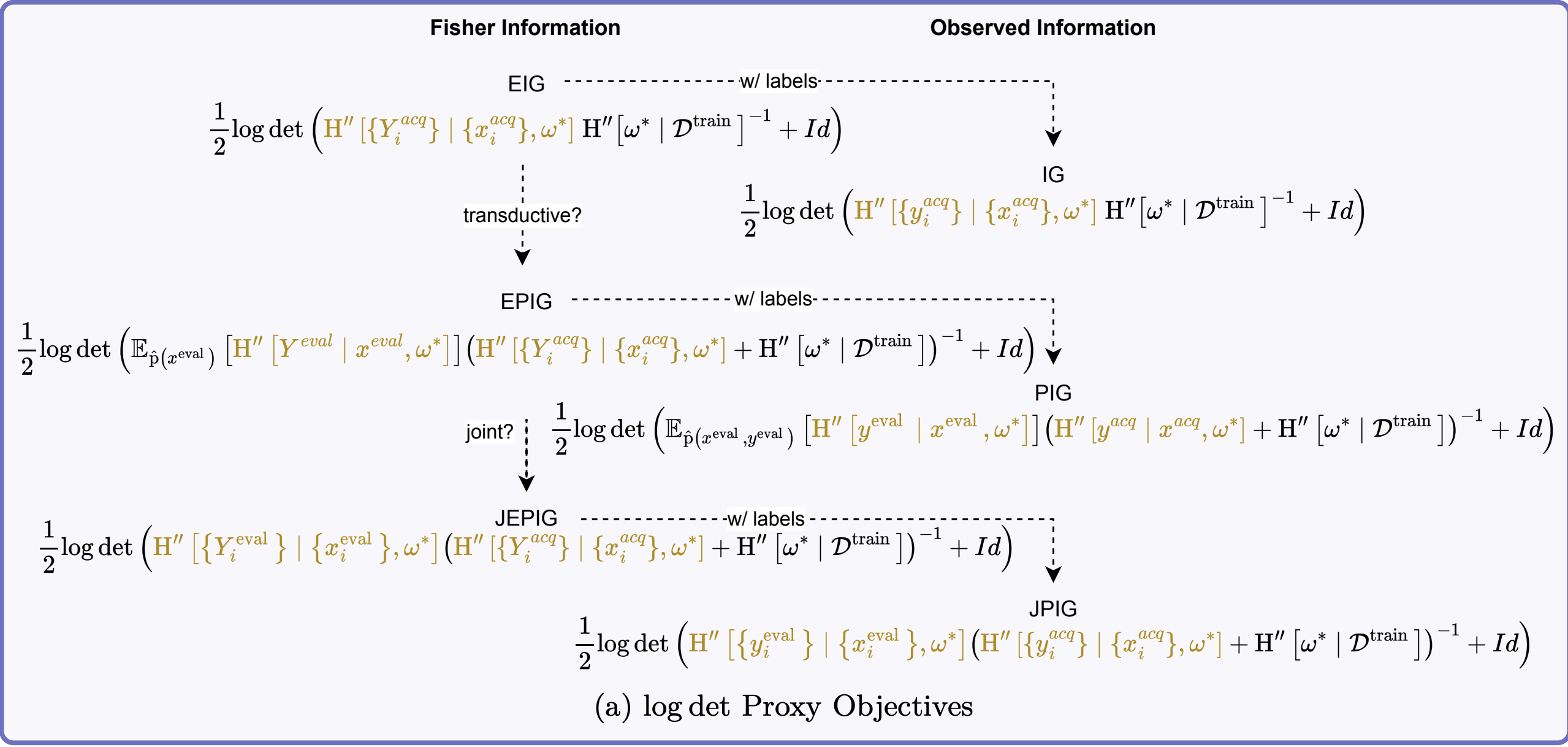
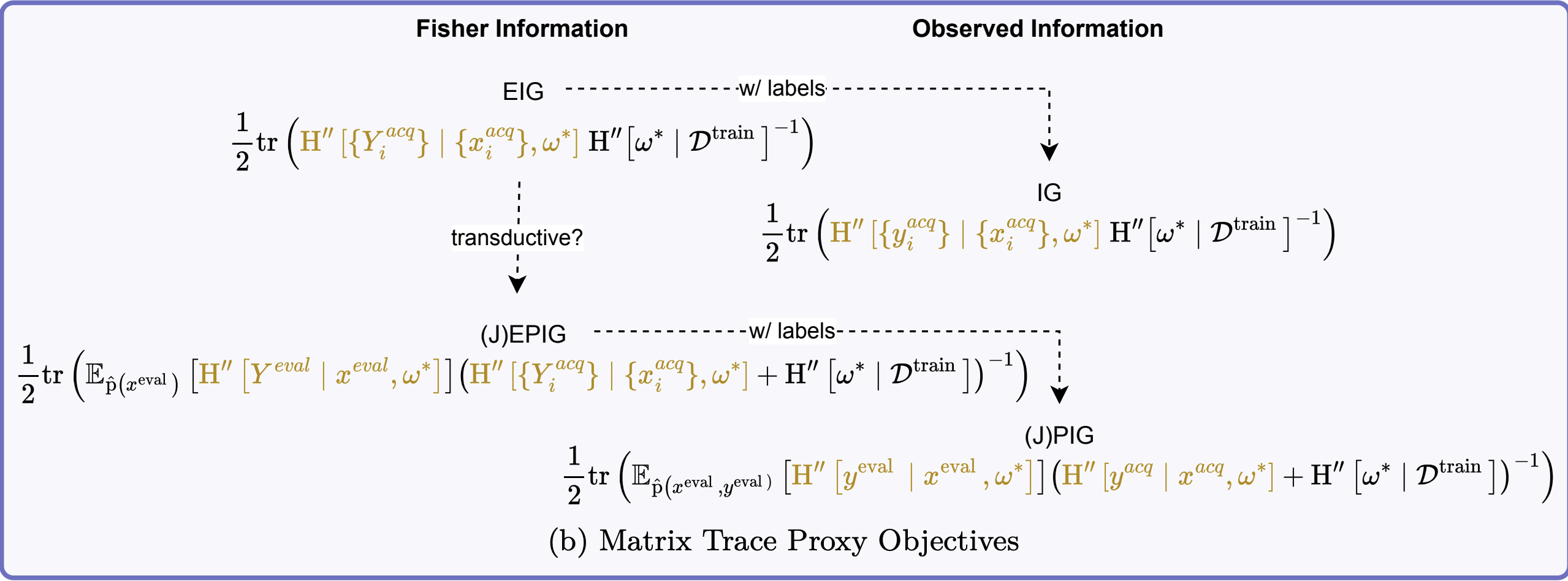
VI. Unified View of Acquisition Functions

A. Key Information Quantities and FIM Approximations

Non-transductive (comparing across all information quantities):

\[ \begin{aligned} \log \det &\left(\left\{\begin{aligned} \FisherInfo{\Yacqset \given \xacqset, \wstar} & \text{ (EIG, GGN/GLM)} \\ \HofHessian{\yacqset \given \xacqset, \wstar} & \text{ (IG)} \end{aligned}\right\}\right.\\ &\left.\left(\left\{\begin{aligned} \FisherInfo{\Yset \given \xset, \wstar} & \text{ GGN/GLM} \\ \HofHessian{\yset \given \xset, \wstar} & \end{aligned}\right\} + \HofHessian{\wstar}\right)^{-1} + I\right) \end{aligned} \]

B. Connecting Popular Methods

• Many recent methods unknowingly approximate the same information-theoretic quantities
• The differences lie in computational approximations, not fundamental objectives
• Let’s see how BADGE, BAIT, PRISM, and others fit into our framework

C. Batch Active Learning by Diverse Gradient Embeddings

(J. T. Ash et al. 2019)

• Uses k-means++ on gradient embeddings using hard pseudo-labels

• k-means++ approximately maximizes log-determinant (k-DPP)

  \[ \log \det(\similarityMatrix{}{\Dacq \given \wstar}) \approx \MIof{\W; \Yacqset \given \xacqset} \]

D. BAIT (J. Ash et al. 2021)

• Directly implements trace approximation of (J)EPIG:

  \[ \begin{aligned} \arg\min_{\xacqset} \tr &\left( (\FisherInfo{\Yacqset \given \xacqset, \wstar} + \FisherInfo{\Ytrain \given \xtrain, \wstar} \right.\\ &\left. + \lambda I)^{-1} \FisherInfo{\Yevalset \given \xevalset, \wstar} \right) \end{aligned} \]

• Uses last-layer Fisher information

• Transductive: uses evaluation set \(\xevalset\) (typically the pool set)

• Revealed: transductive active learning

E. PRISM/SIMILAR: Submodular Methods

(Kothawade et al. 2021)

• Use log-determinant of similarity matrices as “information functions”
• Best results with: \(\log \det(\similarityMatrix{}{\Dacq \given \wstar})\)
• This objective exactly matches our EIG approximation with uninformative prior!

For transductive objectives (LogDetMI): \[ \begin{aligned} &\log \det \similarityMatrix{}{\Dacq \given \wstar} \\ &\quad - \log \det \left(\similarityMatrix{}{\Dacq \given \wstar} - \similarityMatrix{}{\Dacq ; \Deval \given \wstar} \similarityMatrix{}{\Deval \given \wstar}^{-1} \similarityMatrix{}{\Deval ; \Dacq \given \wstar}\right) \end{aligned} \]

This approximates JEPIG!

F. Gradient Length Methods (EGL, GraNd)

• Use \(\|\nabla_\w \mathcal{L}\|^2\)
• Trace of one-sample FIM estimate
• Revealed: Diagonal FIM approximation

Important

Both connect to information gain through diagonal FIM approximations!

VIII. Implications

A. The Unification

• BADGE \(\approx\) EIG with uninformative prior
• BAIT \(\approx\) EPIG with trace approximation
  
• PRISM/SIMILAR (LogDet) \(\approx\) EIG/EPIG
• EGL/GraNd \(\approx\) EIG/IG with diagonal approximation

All are approximating the same few information-theoretic quantities!

B. What This Means

• Conceptual clarity: Seemingly different methods target the same objectives
• Cross-pollination: Improvements in one method may transfer to others
• Principled analysis: We can now understand why methods work or fail

Example: Trace approximations ignore batch redundancies → pathologies

C. Weight Space vs Prediction Space

• Weight space (BADGE, BAIT, etc.):
  • ✓ Computationally efficient
  • ✗ Gaussian approximation quality
  • ✗ May break in low-data regimes
• Prediction space (BALD, BatchBALD):
  • ✓ More accurate information estimates
  • ✗ Combinatorial explosion for batches
  • ✗ Requires multiple model samples

Empirical Validation

1. MNIST at 80 random samples (Kirsch and Gal 2022)
2. Batch active learning for regression (Holzmüller et al. 2023; Kirsch 2023)

MNIST at 80 Random Samples

High rank correlation between methods:

• BALD vs EIG (LogDet): ~0.95
• EPIG (Prediction) vs EPIG (LogDet): ~0.92

Weight-space methods preserve relative ranking!

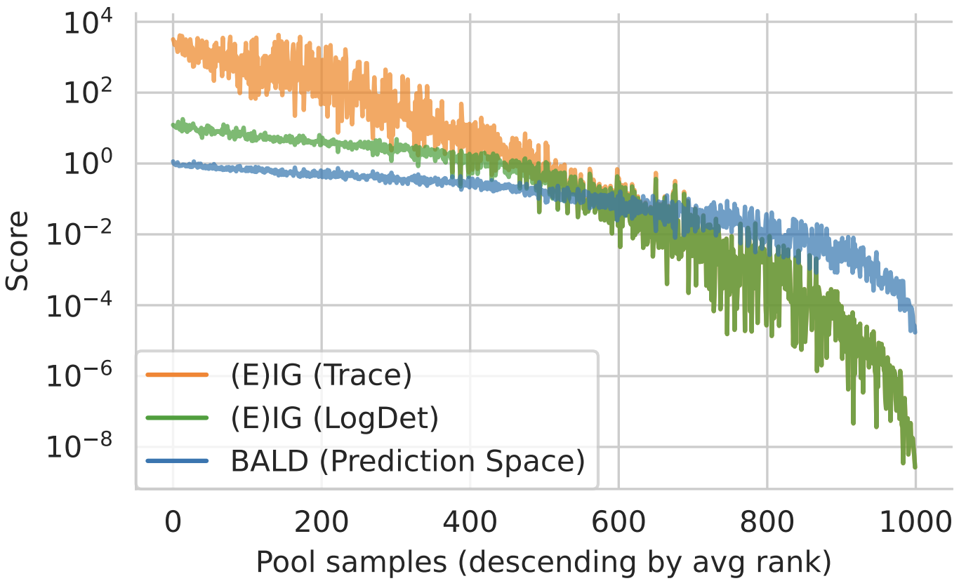
Figure 2: EIG Approximations. Trace and log det approximations match for small scores. They diverge for large scores. Qualitatively, the order matches the prediction-space approximation using BALD with MC dropout.

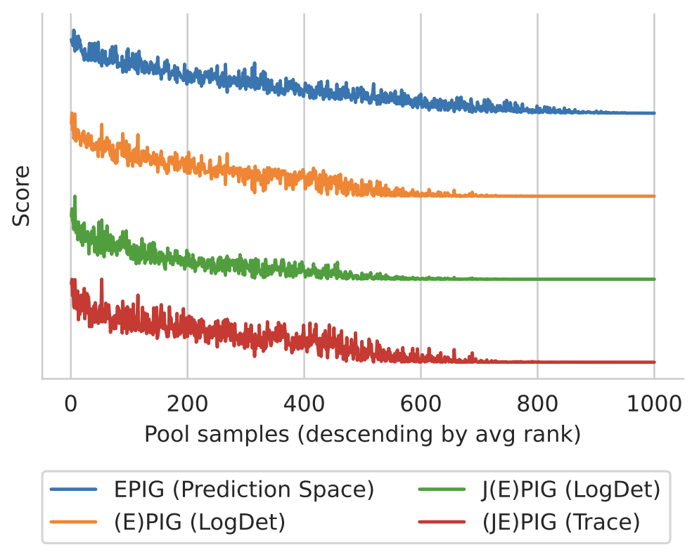
Figure 3: (J)EPIG Approximations (Normalized). The scores match qualitatively. Note we have reversed the ordering for the proxy objectives for JEPIG and EPIG as they are minimized while EPIG is maximized.

Black-box Batch Active Learning for Regression

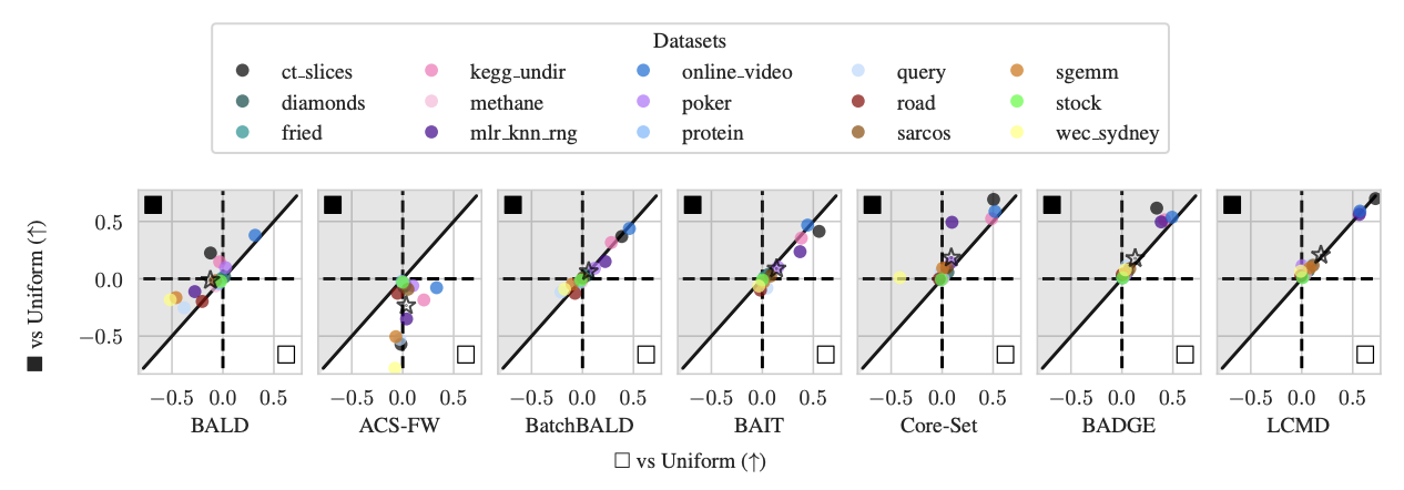
Figure 4: Average Logarithmic RMSE by regression datasets for DNNs: Black-box/prediction-space ■ vs white-box/weight-space □ (vs Uniform). Improvement of the white-box □ method over the uniform baseline on the x-axis and the improvement of the black-box ■ method over the uniform baseline on the y-axis. The average over all datasets is marked with a star ⋆.

D. Open Questions

1. Better approximations: Can we improve beyond hard pseudo-labels?
2. Batch selection: Is BAIT’s forward-backward heuristic generally useful?
3. Beyond last layer: Principled full-network FIM approximations?
4. Empirical validation: When do approximations diverge in practice?

E. Practical Takeaways

• When you see gradient-based AL methods, think “FIM approximation”
• LogDet objectives often work best because they approximate proper information quantities
• Trace approximations = dangerous for batch acquisition
• Last-layer approaches work well with pre-trained models

F. The Bigger Picture

Important

The “informativeness” that various methods try to capture collapses to the same information-theoretic quantities known since (Lindley 1956; MacKay 1992).

Understanding these connections allows us to build better, more principled active learning methods.

Questions & Discussion

Appendix

Ash, Jordan T, Chicheng Zhang, Akshay Krishnamurthy, John Langford, and Alekh Agarwal. 2019. “Deep Batch Active Learning by Diverse, Uncertain Gradient Lower Bounds.” ICLR.

Ash, Jordan, Surbhi Goel, Akshay Krishnamurthy, and Sham Kakade. 2021. “Gone Fishing: Neural Active Learning with Fisher Embeddings.” NeurIPS.

Holzmüller, David, Viktor Zaverkin, Johannes Kästner, and Ingo Steinwart. 2023. “A Framework and Benchmark for Deep Batch Active Learning for Regression.” JMLR.

Houlsby, Neil, Ferenc Huszár, Zoubin Ghahramani, and Máté Lengyel. 2011. “Bayesian Active Learning for Classification and Preference Learning.” arXiv Preprint arXiv:1112.5745.

Kirsch, Andreas. 2023. “Black-Box Batch Active Learning for Regression.” TMLR.

Kirsch, Andreas, and Yarin Gal. 2022. “Unifying Approaches in Active Learning and Active Sampling via Fisher Information and Information-Theoretic Quantities.” TMLR.

Kothawade, Suraj, Nathan Beck, Krishnateja Killamsetty, and Rishabh Iyer. 2021. “Similar: Submodular Information Measures Based Active Learning in Realistic Scenarios.” Advances in Neural Information Processing Systems 34: 18685–97.

Lindley, Dennis V. 1956. “On a Measure of the Information Provided by an Experiment.” The Annals of Mathematical Statistics 27 (4): 986–1005.

MacKay, David JC. 1992. “Information-Based Objective Functions for Active Data Selection.” Neural Computation 4 (4): 590–604.