Submodularity & Batch Acquisition

(BatchBALD & Stochastic Batch Acquisition)

Why Batch Acquisition?

\[ \require{mathtools} \DeclareMathOperator{\opExpectation}{\mathbb{E}} \newcommand{\E}[2]{\opExpectation_{#1} \left [ #2 \right ]} \newcommand{\simpleE}[1]{\opExpectation_{#1}} \newcommand{\implicitE}[1]{\opExpectation \left [ #1 \right ]} \DeclareMathOperator{\opVar}{\mathrm{Var}} \newcommand{\Var}[2]{\opVar_{#1} \left [ #2 \right ]} \newcommand{\implicitVar}[1]{\opVar \left [ #1 \right ]} \newcommand\MidSymbol[1][]{% \:#1\:} \newcommand{\given}{\MidSymbol[\vert]} \DeclareMathOperator{\opmus}{\mu^*} \newcommand{\IMof}[1]{\opmus[#1]} \DeclareMathOperator{\opInformationContent}{H} \newcommand{\ICof}[1]{\opInformationContent[#1]} \newcommand{\xICof}[1]{\opInformationContent(#1)} \newcommand{\sicof}[1]{h(#1)} \DeclareMathOperator{\opEntropy}{H} \newcommand{\Hof}[1]{\opEntropy[#1]} \newcommand{\xHof}[1]{\opEntropy(#1)} \DeclareMathOperator{\opMI}{I} \newcommand{\MIof}[1]{\opMI[#1]} \DeclareMathOperator{\opTC}{TC} \newcommand{\TCof}[1]{\opTC[#1]} \newcommand{\CrossEntropy}[2]{\opEntropy(#1 \MidSymbol[\Vert] #2)} \DeclareMathOperator{\opKale}{D_\mathrm{KL}} \newcommand{\Kale}[2]{\opKale(#1 \MidSymbol[\Vert] #2)} \DeclareMathOperator{\opJSD}{D_\mathrm{JSD}} \newcommand{\JSD}[2]{\opJSD(#1 \MidSymbol[\Vert] #2)} \DeclareMathOperator{\opp}{p} \newcommand{\pof}[1]{\opp(#1)} \newcommand{\pcof}[2]{\opp_{#1}(#2)} \newcommand{\hpcof}[2]{\hat\opp_{#1}(#2)} \DeclareMathOperator{\opq}{q} \newcommand{\qof}[1]{\opq(#1)} \newcommand{\qcof}[2]{\opq_{#1}(#2)} \newcommand{\varHof}[2]{\opEntropy_{#1}[#2]} \newcommand{\xvarHof}[2]{\opEntropy_{#1}(#2)} \newcommand{\varMIof}[2]{\opMI_{#1}[#2]} \DeclareMathOperator{\opf}{f} \newcommand{\fof}[1]{\opf(#1)} \newcommand{\indep}{\perp\!\!\!\!\perp} \newcommand{\Y}{Y} \newcommand{\y}{y} \newcommand{\X}{\boldsymbol{X}} \newcommand{\x}{\boldsymbol{x}} \newcommand{\w}{\boldsymbol{\theta}} \newcommand{\W}{\boldsymbol{\Theta}} \newcommand{\wstar}{\boldsymbol{\theta^*}} \newcommand{\D}{\mathcal{D}} \newcommand{\HofHessian}[1]{\opEntropy''[#1]} \newcommand{\specialHofHessian}[2]{\opEntropy''_{#1}[#2]} \newcommand{\HofJacobian}[1]{\opEntropy'[#1]} \newcommand{\specialHofJacobian}[2]{\opEntropy'_{#1}[#2]} \newcommand{\indicator}[1]{\mathbb{1}\left[#1\right]} \]

Real-World Impact

Labeling data is expensive ($200+/hour for medical experts)
Need to request labels in batches for efficiency
Naive batch selection often wastes resources

What You’ll Learn Today

After this lecture, you’ll be able to:

Understand why naive batch acquisition fails
Apply information theory to batch selection
Use submodularity for efficient algorithms
Implement BatchBALD in practice

Common Misconceptions

Warning

Batch acquisition is NOT:

Simply selecting top-k points independently
Only about computational efficiency
Limited to specific acquisition functions

Batch Acquisition

Top-K Algorithm

Pseudocode

def naive_batch_acquisition(pool_set, batch_size, model):
    # Score all points independently 
    scores = []
    for x in pool_set:
        score = acquisition_function(x, model)
        scores.append((x, score))
    
    # Sort by score and take top-k
    scores.sort(key=lambda x: x[1], reverse=True)
    selected = [x for x,_ in scores[:batch_size]]
    
    return selected

The Problem with Top-K

Selects points independently
Ignores redundancy between points
Can waste labeling budget
Gets worse with larger batch sizes

Redundancy Issue

Consider MNIST digits:

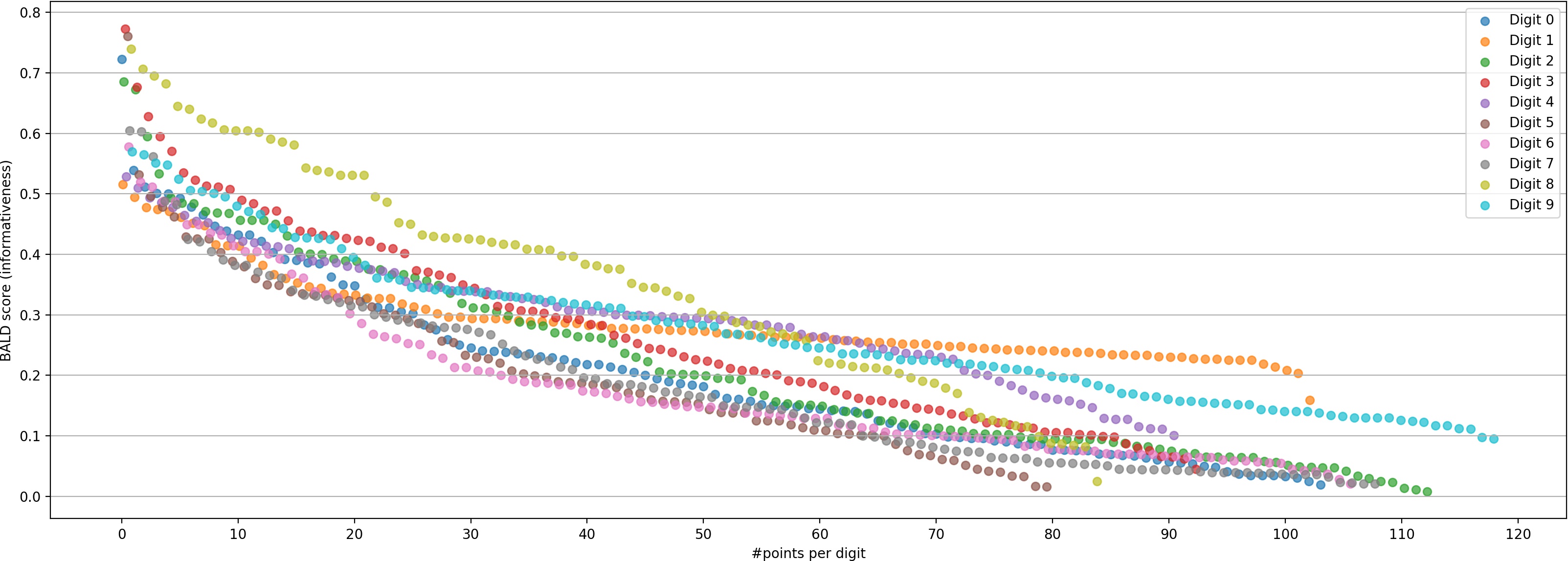
Note

Top-K selects many “8”s
All provide similar information overall vs other digits
Wastes labeling budget
Better to select diverse examples

Simple Baseline

Bucket by predicted class
Select examples by highest acquisition function score in each bucket round-robin.

Batch Size Effect

Small Batch Size

Easier to contain only similar points
More vulnerable to local redundancy
May need more acquisition rounds

Large Batch Size

Unlikely to contain only similar points
Natural diversity through size
More expensive labelling

Promise of Good Batch Acquisition

Saving Time and Labelling Cost

Information-Theoretic Perspective

BALD (≙ EIG)

For random variables $\Y$ (labels) and $\W$ (model parameters):

\[ \MIof{\Y; \W \given \x, \D} = \Hof{\Y \given \x, \D} - \E{\pof{\w \given \D}}{\Hof{\Y \given \x, \w}} \]

Note

This measures how much knowing the model parameters reduces our uncertainty about labels

Top-K Sum Equivalence

Let $\mathcal{A}_k$ be a batch of $k$ points.

Taking the top-k points by score is equivalent to:

\[ \arg \max_{\mathcal{A}_k \subseteq \mathcal{P}, |\mathcal{A}_k| = k} \sum_{x \in \mathcal{A}_k} \MIof{\Y; \W \given x, \D} \]

Key Insight

This shows why Top-K fails: it assumes information from each point adds independently!

Top-K Intuition

\[ \sum_{x \in \mathcal{A}_k} \MIof{\Y; \W \given x, \D} \]

Batch Intuition

How can we avoid double-counting information?

We want:

\[ \IMof{\W \cap (\cup_{x \in \mathcal{A}_k} \Y \given \x)} \]

I-Diagram $\Rightarrow$ Information Quantity

\[ \IMof{\W \cap (\cup_{x \in \mathcal{A}_k} \Y \given \x)} \]

\[ \implies \equiv \MIof{\Y_1, .., \Y_k; \W \given \x_1, .., \x_k, \D}. \]

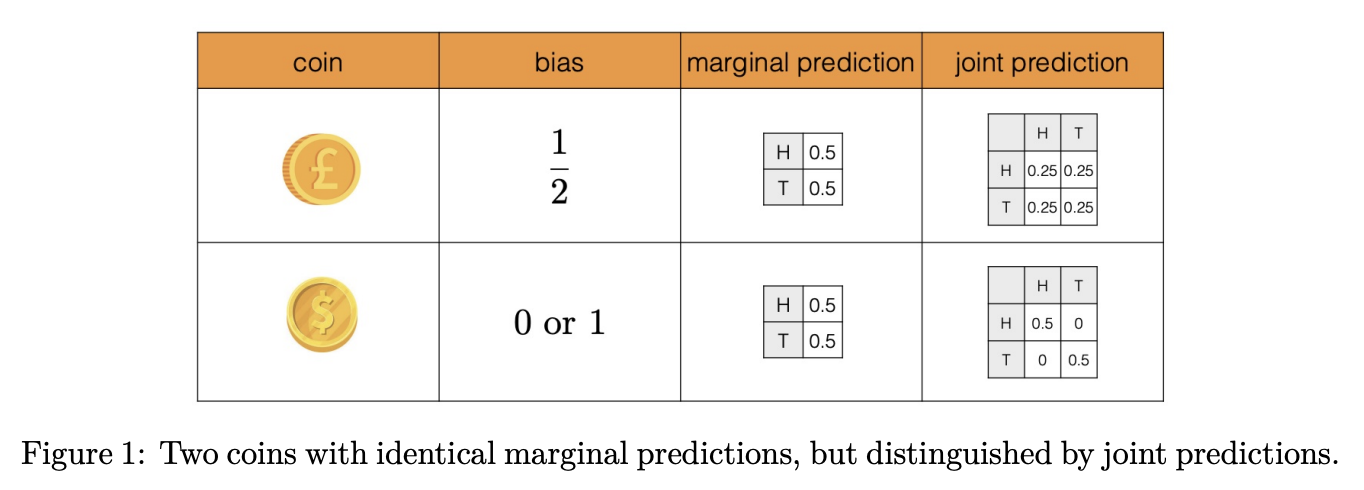
Joint Mutual Information

Definition 1 (BatchBALD) BatchBALD is the mutual information between the model parameters and the joint predictions of a batch of points:

\[ \MIof{\Y_1, .., \Y_k; \W \given \x_1, .., \x_k, \D} \]

Comparison

BALD

Scores independently
Double counts
$\sum_{i} \MIof{\Y_i; \W \given \x_i, \D}$

BatchBALD

Scores jointly
Accounts for redundancy
$\MIof{\Y_1, .., \Y_k; \W \given \x_1, .., \x_k, \D}$

Acquisition Function

\[\arg \max_{\mathcal{A}_k \subseteq \mathcal{P}, |\mathcal{A}_k| = k} \MIof{\Y_1, .., \Y_k; \W \given \x_1, .., \x_k, \D}\]

Problem: combinatorial search over all subsets!

🙀😱

What’s a cheap way to find a batch?

Greedy Optimization

def greedy_batch_acquisition(pool_set, k, acquisition_fn):
    batch = []
    remaining = set(pool_set)
    
    for _ in range(k):
        # Find point that maximizes marginal gain
        best_x = max(remaining, 
                    key=lambda x: acquisition_fn(batch + [x]))
        
        batch.append(best_x)
        remaining.remove(best_x)
    
    return batch

Key Properties

Simple to implement
Works well in practice

Guarantees

It actually works well in practice and achieves approximately a \[ 1-\frac{1}{e} \approx 0.63 \] approximation ratio of the optimal batch!

Submodularity

Greedy optimization of submodular functions yields a \[ 1-\frac{1}{e} \approx 0.63 \] approximation of the optimum!

What is Submodularity?

Submodularity captures “diminishing returns”:

Adding elements to larger sets gives less benefit

Submodularity Visualization

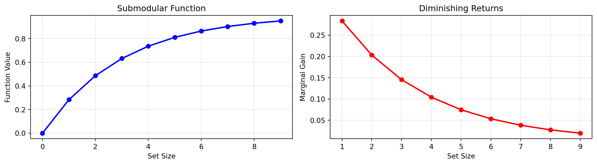
Left: Total value increases sublinearly
Right: Marginal gain decreases with set size

Formal Definition

Nemhauser, Wolsey, and Fisher (1978):

Definition 2 A set function $f$ is submodular when $\forall A, B$:

\[ f(A \cup B) + f(A \cap B) \leq f(A) + f(B). \]

More Intuitive Definition?

Intuitively:

Adding elements to larger sets gives fewer benefits
For $X$ and $Y_1 \subseteq Y_2$, such that $X$ and $Y_2$ are disjoint ($X \cap Y_2 = \emptyset$):
- “$f(X \given Y_2) \leq f(X \given Y_1)$.”
- Formal: \[ f(X \cup Y_2) - f(Y_2) \leq f(X \cup Y_1) - f(Y_1). \]

Formal More Intuitive Definition

Theorem 1 For $X$ and $Y_1 \subseteq Y_2$, such that $X$ and $Y_2$ are disjoint ($X \cap Y_2 = \emptyset$), $f$ is submodular iff:

\[ f(X \cup Y_2) - f(Y_2) \leq f(X \cup Y_1) - f(Y_1). \]

If we define the marginal gain of adding $X$ to $Y$:

\[ \Delta(X \given Y) \coloneqq f(X \cup Y) - f(Y), \]

then this is equivalent to:

\[ \Delta(X \given Y_1) \leq \Delta(X \given Y_2). \]

Proof of Equivalence

Proof (Formal Definition $\implies$ Intuitive Definition).

Assume $f$ is submodular as per the formal definition:

\[ f(A \cup B) + f(A \cap B) \leq f(A) + f(B). \]
For $X$ and $Y_1 \subseteq Y_2$, such that $X$ and $Y_2$ are disjoint ($X \cap Y_2 = \emptyset$), let:
- $A \coloneqq X \cup Y_1$
- $B \coloneqq Y_2$
Given that $Y_1 \subseteq Y_2$ and $X \cap Y_2 = \emptyset$, we have:
- $A \cup B = X \cup Y_1 \cup Y_2 = X \cup Y_2$
- $A \cap B = (X \cup Y_1) \cap Y_2 = (X \cap Y_2) \cup (Y_1 \cap Y_2) = Y_1$
Starting from the formal submodular inequality:

\[ \begin{aligned} f(A \cup B) + f(A \cap B) &\leq f(A) + f(B) \\ \iff f(X \cup Y_2) + f(Y_1) &\leq f(X \cup Y_1) + f(Y_2) \\ \iff f(X \cup Y_2) - f(Y_2) &\leq f(X \cup Y_1) - f(Y_1). \end{aligned} \]

This matches the intuitive definition. $\square$

Proof (Intuitive Definition $\implies$ Formal Definition).

Assume $f$ satisfies the intuitive definition:

\[ f(X \cup Y_2) - f(Y_2) \leq f(X \cup Y_1) - f(Y_1), \]

for all $X$ and $Y_1 \subseteq Y_2$, such that $X$ and $Y_2$ are disjoint ($X \cap Y_2 = \emptyset$).
Let’s consider arbitrary sets $A$ and $B$. Define:
- $X \coloneqq A \setminus B$
- $Y_1 \coloneqq A \cap B$
- $Y_2 \coloneqq B$
Now compute:
- $X \cup Y_1 = (A \setminus B) \cup (A \cap B) = A$
- $X \cup Y_2 = (A \setminus B) \cup B = A \cup B$
Observe that:
- $X \cap Y_2 = (A \setminus B) \cap B = \emptyset$
- $Y_1 \subseteq Y_2$
Thus, the intuitive definition implies:

\[ \begin{aligned} f(X \cup Y_2) - f(Y_2) &\leq f(X \cup Y_1) - f(Y_1) \\ \iff f(A \cup B) - f(B) &\leq f(A) - f(A \cap B) \\ \iff f(A \cup B) + f(A \cap B) &\leq f(A) + f(B). \end{aligned} \]

This matches the formal definition. $\square$

Simpler Definition

But wait, there is more—we can simplify this further:

Theorem 2 For any $Y_1 \subseteq Y_2$ and $e \notin Y_2$, $f$ is submodular iff:

\[ f(Y_2 \cup \{e\}) - f(Y_2) \leq f(Y_1 \cup \{e\}) - f(Y_1). \]

That is:

\[ \Delta(e \given X) \leq \Delta(e \given Y). \]

Proof

$\implies$ follows immediately from the previous definition.
$\impliedby$:
1. We assume that for any $Y_1 \subseteq Y_2$ and $e \notin Y_2$:
  
  \[ \Delta(e \given Y_2) \leq \Delta(e \given Y_1). \]
2. For $X$ and $Y_1 \subseteq Y_2$, such that $X$ and $Y_2$ are disjoint ($X \cap Y_2 = \emptyset$), let:
  
  \[ \begin{aligned} S &\coloneqq Y_2 \setminus Y_1, \\ S &\coloneqq \{s_1, \ldots, s_n\}, \\ S_k &\coloneqq \{s_1, \ldots, s_k\} \subseteq S. \end{aligned} \]
3. For all $k$, we have:
  
  \[ \begin{aligned} \Delta(s_k \given X \cup Y_1 \cup S_{k-1}) &\leq \Delta(s_k \given Y_1 \cup S_{k-1}), \end{aligned} \]
  
  as $Y_1 \cup S_{k-1} \subseteq X \cup Y_1 \cup S_{k-1}$.
Telescoping

Telescoping is a technique where terms in a sequence cancel out except for the first and last terms. The name comes from how a telescope’s segments collapse into each other.
1. Using telescoping, we get:
  
  \[ \begin{aligned} \sum_{k=1}^{n} \Delta(s_k \given X \cup Y_1 \cup S_{k-1}) &\leq \sum_{k=1}^{n} \Delta(s_k \given Y_1 \cup S_{k-1}) \\ \iff \sum_{k=1}^{n} f(X \cup Y_1 \cup S_{k-1} \cup \{s_k\}) &\\ - f(X \cup Y_1 \cup S_{k-1}) &\leq \sum_{k=1}^{n} f(Y_1 \cup S_{k-1} \cup \{s_k\}) \\ &\hphantom{\leq} - f(Y_1 \cup S_{k-1}) \\ \iff \sum_{k=1}^{n} f(X \cup Y_1 \cup S_{k}) &\\ - f(X \cup Y_1 \cup S_{k-1}) &\leq \sum_{k=1}^{n} f(Y_1 \cup S_{k}) \\ & \hphantom{\leq} - f(Y_1 \cup S_{k-1}) \\ \iff f(X \cup Y_1 \cup S) &\\ - f(X \cup Y_1) &\leq f(Y_1 \cup S) - f(Y_1) \\ \iff f(X \cup Y_2) &\\ - f(X \cup Y_1) &\leq f(Y_2) - f(Y_1), \end{aligned} \]
  
  where we have used that $Y_2 = Y_1 \cup S \leftrightarrow S = Y_2 \setminus Y_1$.
2. Rearranging, we get:
  
  \[ f(X \cup Y_2) - f(Y_2) \leq f(X \cup Y_1) - f(Y_1). \]
  
  $\square$

Summary

This characterizes submodularity in terms of marginal gains:

\[ \begin{aligned} f &\text{ is submodular} \\ \iff f(A \cup B) + f(A \cap B) &\leq f(A) + f(B) \\ \iff \Delta(X \given Y_2) &\leq \Delta(X \given Y_1) \\ \iff \Delta(e \given Y_2) &\leq \Delta(e \given Y_1). \end{aligned} \]

for $Y_1 \subseteq Y_2$ and $e \notin Y_2$ and $X \cap Y_2 = \emptyset$.

$1 - \frac{1}{e}$ Optimality

Theorem 3 For a monotone submodular function $f$ with $f(\emptyset) = 0$, the greedy algorithm achieves at least:

\[ f(\mathcal{A}_k^{\text{greedy}}) \geq \left(1 - \frac{1}{e}\right) f(\mathcal{A}_k^*) \]

where $\mathcal{A}_k^*$ is the optimal set of size $k$.

Key Insights

Greedy selection achieves ≈63% of optimal value
Holds even for very large search spaces

Monotone Submodular Functions

Definition 3 A set function $f: 2^V \rightarrow \mathbb{R}$ is monotone if for all $A \subseteq B \subseteq V$:

\[ f(A) \leq f(B) \]

Intuition

Adding elements never hurts $\leftrightarrow$ non-negative gains!
Function value can only increase
Different from diminishing returns!

Common Confusion

Submodularity: diminishing returns
Monotonicity: always increasing
Both needed for greedy guarantees!

Questions

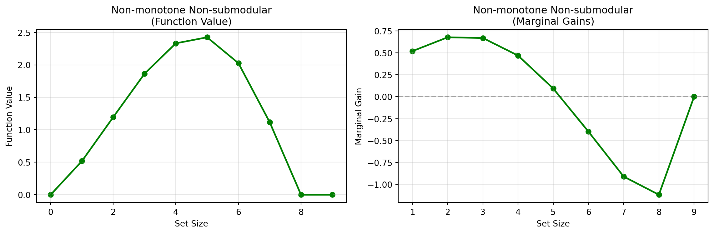
What does a non-monotone submodular function look like?
What does a non-monotone non-submodular function look like?

Submodular Non-/Monotone

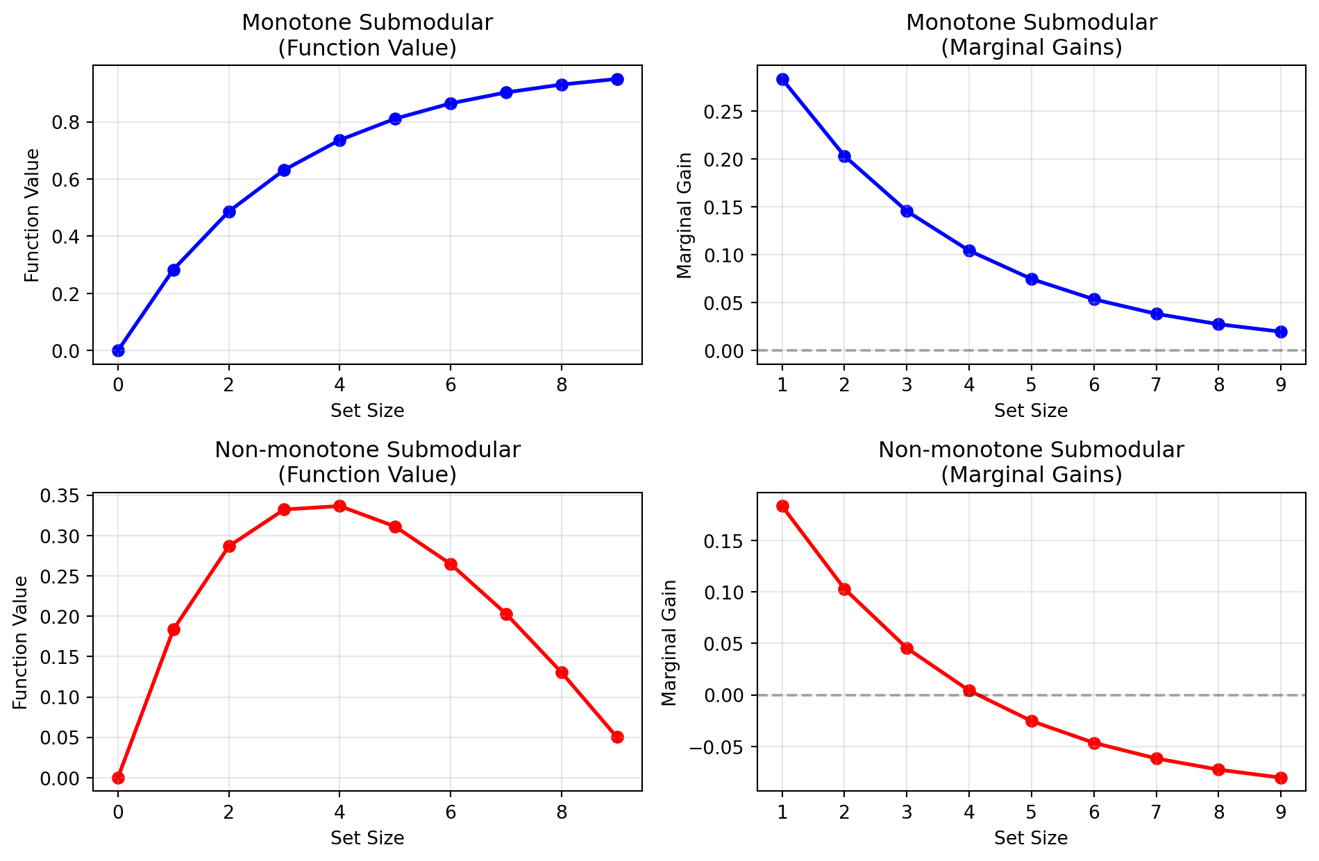
Non-Submodular Non-Monotone

Optimality Proof

Statement

Let $f: 2^{\mathcal{V}} \rightarrow \mathbb{R}_{\geq 0}$ be a monotone (i.e., $f(A) \leq f(B)$ whenever $A \subseteq B$), and submodular function with $f(\emptyset) = 0$ defined over a finite ground set $\mathcal{V}$.

Our goal is to select a subset $S \subseteq \mathcal{V}$ of size $k$ that maximizes $f(S)$:

\[ S^* = \arg\max_{|S| \leq k} f(S). \]

Greedy Algorithm

The greedy algorithm constructs a set $S_{\text{greedy}}$ by starting with $S_0 = \emptyset$ and iteratively adding elements:

\[ S_{i} = S_{i-1} \cup \{ e_i \}, \]

where $e_i$ is chosen to maximize the marginal gain:

\[ \begin{aligned} e_i &\coloneqq \arg\max_{e \in \mathcal{V} \setminus S_{i-1}} \left[ f(S_{i-1} \cup \{ e \}) - f(S_{i-1}) \right] \\ &= \arg\max_{e \in \mathcal{V} \setminus S_{i-1}} \Delta(e \mid S_{i-1}). \end{aligned} \]

Goal

We will show that:

\[ f(S_{\text{greedy}}) \geq \left( 1 - \frac{1}{e} \right) f(S^*). \]

Key Concepts

Marginal Gain: The benefit of adding an element $e$ to a set $A$:

\[ \Delta(e \mid A) \coloneqq f(A \cup \{ e \}) - f(A). \]
Submodularity: Diminishing returns property, i.e., for $A \subseteq B$, we have:

\[ \Delta(e \mid A) \geq \Delta(e \mid B). \]

Proof Sketch

Bounding the Marginal Gain

At each iteration $i$:

\[ \Delta(e_i \mid S_{i-1}) \geq \frac{1}{k} \left[ f(S^*) - f(S_{i-1}) \right]. \]
Recursive Inequality

Update the function value:

\[ f(S_i) \geq f(S_{i-1}) + \frac{1}{k} \left[ f(S^*) - f(S_{i-1}) \right]. \]
Unfolding the Recursion

After $k$ iterations:

\[ f(S_{\text{greedy}}) \geq \left( 1 - \left( 1 - \frac{1}{k} \right)^k \right) f(S^*). \]
Limit Evaluation

As $k$ increases:

\[ \left( 1 - \frac{1}{k} \right)^k \leq \frac{1}{e}, \]

so:

\[ f(S_{\text{greedy}}) \geq \left( 1 - \frac{1}{e} \right) f(S^*). \]

Proof of $\left(1 - \frac{1}{e}\right)$-Optimality

Step 1: Bounding the Marginal Gain

At iteration $i$, consider the optimal set $S^*$ and the current greedy set $S_{i-1}$.
Define $R \coloneqq S^* \setminus S_{i-1}$.
Since $|S^*| = k$, we have $|R| \leq k$.
By submodularity and the fact that $f$ is monotone:

\[ \begin{align*} f(S^*) - f(S_{i-1}) &\leq f(S_{i-1} \cup R) - f(S_{i-1}) \\ &\leq \sum_{e \in R} \Delta(e \mid S_{i-1}). \end{align*} \tag{1}\]

Explanation:
- First inequality from monotonicity.
- Second inequality from submodularity after telescoping:
  
  \[ \begin{aligned} &f(S_{i-1} \cup R) - f(S_{i-1}) \\ &\quad = \sum_{i=1}^{|R|} f(S_{i-1} \cup \{r_1, \ldots, r_i\}) \\ &\quad \phantom{= \sum} - f(S_{i-1} \cup \{r_1, \ldots, r_{i-1}\}) \\ &\quad = \sum_{i=1}^{|R|} \Delta(r_i \mid S_{i-1} \cup \{r_1, \ldots, r_{i-1}\}) \\ &\quad \leq \sum_{i=1}^{|R|} \Delta(r_i \mid S_{i-1})\\ &\quad = \sum_{e \in R} \Delta(e \mid S_{i-1}). \end{aligned} \]
Since the greedy choice $e_i$ maximizes $\Delta(e \mid S_{i-1})$:

\[ \begin{aligned} \Delta(e_i \mid S_{i-1}) &\geq \frac{1}{|R|} \sum_{e \in R} \Delta(e \mid S_{i-1}) \\ &\geq \frac{1}{k} \left[ f(S^*) - f(S_{i-1}) \right]. \end{aligned} \]

Explanation:
- First inequality from maximality:
  
  \[ \Delta(e_i \mid S_{i-1}) \geq \Delta(e \mid S_{i-1}), \]
- and summing over all $e \in R$:
  
  \[ |R| \Delta(e_i \mid S_{i-1}) \geq \sum_{e \in R} \Delta(e \mid S_{i-1}). \]
- Second inequality follows from $|R| \leq k$ and Equation 1 above.

Step 2: Recursive Inequality

From the above bound:

\[ \begin{align*} f(S_i) &= f(S_{i-1}) + \Delta(e_i \mid S_{i-1}) \\ &\geq f(S_{i-1}) + \frac{1}{k} \left[ f(S^*) - f(S_{i-1}) \right] \\ &= \left( 1 - \frac{1}{k} \right) f(S_{i-1}) + \frac{1}{k} f(S^*). \end{align*} \]

Step 3: Unfolding the Recursion

Define $\gamma_i \coloneqq f(S^*) - f(S_i)$.
Then:

\[ \gamma_i \leq \left( 1 - \frac{1}{k} \right) \gamma_{i-1}. \]

Note

Explanation:

We subtract the previous inequality

\[ f(S_i) \geq \left( 1 - \frac{1}{k} \right) f(S_{i-1}) + \frac{1}{k} f(S^*) \]

from $f(S^*)$
which yields:

\[ \begin{aligned} &f(S^*) - f(S_i) \\ &\quad \leq f(S^*) - \left[ \left( 1 - \frac{1}{k} \right) f(S_{i-1}) + \frac{1}{k} f(S^*) \right] \\ &\quad = \left( 1 - \frac{1}{k} \right) \left[ f(S^*) - f(S_{i-1}) \right]. \end{aligned} \]
which is just the definition of $\gamma_i$ on the LHS and $\gamma_{i-1}$ on the RHS:

\[ \gamma_i \leq \left( 1 - \frac{1}{k} \right) \gamma_{i-1}. \]

By iterating this inequality:

\[ \gamma_k \leq \left( 1 - \frac{1}{k} \right)^k f(S^*). \]

Explanation:
- We start with
  
  \[ \gamma_0 = f(S^*) - f(S_0) = f(S^*), \]
  
  as $f(S_0) = f(\emptyset) = 0$.
- Then we apply the inequality $\gamma_i \leq \left( 1 - \frac{1}{k} \right) \gamma_{i-1}$ iteratively to obtain:
  
  \[ \begin{aligned} \gamma_k &\leq \left( 1 - \frac{1}{k} \right) \left( 1 - \frac{1}{k} \right) \cdots \left( 1 - \frac{1}{k} \right) \gamma_0 \\ &= \left( 1 - \frac{1}{k} \right)^k \gamma_0. \end{aligned} \]
Thus, the greedy solution satisfies:

\[ \begin{aligned} f(S_{\text{greedy}}) &= f(S_k) \\ &= f(S^*) - \gamma_k \\ &\geq f(S^*) \left( 1 - \left( 1 - \frac{1}{k} \right)^k \right). \end{aligned} \]

Explanation:
- We start with $\gamma_k = f(S^*) - f(S_k)$.
- Then we apply the itereated inequality to obtain:
  
  \[ \begin{aligned} f(S^*) - \gamma_k &\geq f(S^*) - \left( 1 - \frac{1}{k} \right)^k f(S^*) \\ &= f(S^*) \left( 1 - \left( 1 - \frac{1}{k} \right)^k \right). \end{aligned} \]

Step 4: Limit Evaluation

Remembering that:

\[ \lim_{k \rightarrow \infty} \left( 1 - \frac{1}{k} \right)^k = \frac{1}{e}, \]
and that:

\[ \left( 1 - \frac{1}{k} \right)^k < \frac{1}{e}, \]
we conclude:

\[ \begin{aligned} f(S_{\text{greedy}}) &\geq \left( 1 - \left( 1 - \frac{1}{k} \right)^k \right) f(S^*) \\ &\geq \left( 1 - \frac{1}{e} \right) f(S^*). \end{aligned} \] $\square$

Summary

The greedy algorithm provides a $\left( 1 - \frac{1}{e} \right)$-approximation to the optimal solution when maximizing a non-negative, monotone, submodular function under a cardinality constraint.

Why?

This result is significant because it guarantees that the greedy approach to batch acquisition in settings like active learning will achieve near-optimal utility, ensuring efficient use of resources.

Submodular BatchBALD

Set

\[ f({\x_1, \ldots, \x_k}) \coloneqq \MIof{\Y_1, \ldots, \Y_k; \W \given \x_1, \ldots, \x_k}. \]

Show:

$f(\emptyset) = 0$
Monotone
Submodular

Marginal Gain

For this definition of $f$, the marginal gain is:

\[ \begin{aligned} \Delta(x_e \mid \x_1, .., \x_k) &= f(\{ \x_1, .., \x_k, \x_e \}) - f(\{ \x_1, .., \x_k \}) \\ &= \MIof{\Y_e, \Y_1, .., \Y_k; \W \given \x_e, \x_1, .., \x_k} \\ &\quad - \MIof{\Y_1, .., \Y_k; \W \given \x_1, .., \x_k} \\ &= \MIof{\Y_e; \W \given \x_e, \Y_1, \x_1, .., \Y_k, \x_k} \\ \end{aligned} \]

Proof (Last Step)

Convince yourself that:

\[ \MIof{A, B; \W \given C} = \MIof{A; \W \given C} + \MIof{B; \W \given A, C}. \]
And then:

\[ \MIof{B; \W \given A, C} = \MIof{A, B; \W \given C} - \MIof{A; \W \given C}. \] $\square$

Proof: $f(\emptyset) = 0$

\[ f(\emptyset) = \MIof{ \emptyset; \W} = 0. \] $\square$

Proof: Monotone

Show that for $A \subseteq B$:

\[ f(A) \leq f(B). \]

Proof.

For $x_1, .., x_n \in \mathcal{P}$ and $1 \le k \le n, k \in \mathbb{N}$:

\[ \begin{aligned} &f(\{ \x_1, .., \x_k \}) \\ &\quad \leq f(\{ \x_1, .., \x_n \}) \\ \iff &\MIof{\Y_1, .., \Y_k; \W \given \x_1, .., \x_k} \\ &\quad \leq \MIof{\Y_1, .., \Y_{n}; \W \given \x_1, .., \x_{n}} \\ \iff &\Hof{\W} - \Hof{\W \given \Y_1, .., \Y_k, \x_1, .., \x_k} \\ &\quad \leq \Hof{\W} - \Hof{\W \given \Y_1, .., \Y_{n}, \x_1, .., \x_{n}} \\ \iff &\Hof{\W \given \Y_1, .., \Y_k, \x_1, .., \x_k} \\ &\quad \geq \Hof{\W \given \Y_1, .., \Y_{n}, \x_1, .., \x_{n}}. \end{aligned} \]
Conditioning reduces entropy.
Thus, $f$ is monotone. $\square$

Alternative:

We notice that

\[ \begin{aligned} &f(\{ \x_1, .., \x_k \}) \leq f(\{ \x_1, .., \x_n \}) \\ \iff &0 \leq \Delta(\x_{k+1}, .., \x_n \mid \x_1, .., \x_k) \\ \iff &0 \leq \MIof{\Y_{k+1}, .., \Y_n; \W \given \x_{k+1}, .., \x_n, \Y_1, .., \Y_k, \x_1, .., \x_k}, \end{aligned} \]

which is true as pairwise mutual information is non-negative. $\square$

Proof: Submodular

For $X$ and $Y_1 \subseteq Y_2$ with $X \cap Y_2 = \emptyset$, we need to show:

\[ \Delta(X \given Y_2) \leq \Delta(X \given Y_1). \]
Notation: We rename these to $A$ and $B_1 \subseteq B_2$ to avoid confusing with the random variables $\X$ and $\Y$. We drop the conditioning on $\x$ and only write the $\Y$ to save space.
We need to show:

\[ \MIof{\Y_{A} ; \W \given \Y_{B_2}} \leq \MIof{\Y_{A} ; \W \given \Y_{B_1}}. \]
Let:

\[ S \coloneqq B_2 \setminus B_1. \]
We can rewrite this as:

\[ \begin{aligned} &\MIof{\Y_{A} ; \W \given \Y_{B_1}} - \MIof{\Y_{A} ; \W \given \Y_{B_2}} \geq 0 \\ \iff &\MIof{\Y_{A} ; \W \given \Y_{B_1}} - \MIof{\Y_{A} ; \W \given \Y_{B_1}, \Y_{S}} \geq 0 \\ \iff &\MIof{\Y_{A} ; \W ; \Y_S \given \Y_{B_1}} \geq 0. \end{aligned} \]
Using the symmetry of the mutual information:

\[ \begin{aligned} 0 &\leq \MIof{\Y_{A} ; \W ; \Y_S \given \Y_{B_1}} \\ &= \MIof{\Y_{A} ; \Y_S; \W \given \Y_{B_1}} \\ &= \MIof{\Y_{A} ; \Y_S \given \W, \Y_{B_1}} - \MIof{\Y_{A} ; \Y_S \given \W, \Y_{B_1}} \\ &= \MIof{\Y_{A} ; \Y_S \given \W, \Y_{B_1}} \ge 0, \end{aligned} \]

because $\MIof{\Y_{A} ; \Y_S \given \W, \Y_{B_1}} = 0$ and the pairwise mutual information is non-negative.
$\MIof{\Y_{A} ; \Y_S \given \W, \Y_{B_1}} = 0$ because:
1. Recall that our probabilistic model is
  
  \[ \pof{\y_1, .., \y_n, \w \given \x_1, .., \x_n} = \pof{\w} \prod_{i=1}^n \pof{\y_i \given \w, \x_i}. \]
2. Thus, for all $i \not=j$: \[ \Y_i \indep \Y_j \given \W, \x_i, \x_j. \]
Thus, $f$ is submodular. $\square$

Summary

$f$ is submodular and monotone, that is

\[ f_{\text{BatchBALD}}({\x_1, \ldots, \x_k}) \coloneqq \MIof{\Y_1, \ldots, \Y_k; \W \given \x_1, \ldots, \x_k}. \]

Note

BatchBALD is submodular, allowing efficient computation despite the combinatorial nature of batch selection

Revisiting the Greedy Algorithm

Given $x_1, \ldots, x_{i-1}$, at each step we find the point $x_i$ that maximizes:

\[ f_{\text{BatchBALD}}({\x_1, \ldots, \x_{i-1}, x_i}). \]
The first ${\x_1, \ldots, \x_{i-1}}$ are already selected and thus fixed.
We can just as well maximize the marginal gain:

\[ \Delta(x \given x_1, \ldots, x_{i-1}) = \MIof{\Y; \W \given x, \Y_1, \x_1, \ldots, \Y_{i-1}, \x_{i-1}}. \]
At each step, we thus maximize the EIG conditioned on the other selected points in expectation (we don’t know the actual labels so we use the predictive distribution and take expectations wrt. the labels!).

BatchBALD in Practice

Key Components

Joint mutual information computation
Efficient caching strategies
MC dropout for uncertainty

Results

Performance Gains

More diverse batch selection
Better data efficiency
State-of-the-art results on standard benchmarks

Computing BatchBALD

Given some samples $\w_1$, …, $\w_k$, we need to compute:

\[ \MIof{\Y_1, \ldots, \Y_n; \W \given \x_1, \ldots, \x_n}. \]

Split

Because predictions are independent given the weights, we have:

\[ \begin{aligned} \MIof{\Y_1, .., \Y_n; \W \given \x_1, .., \x_n} &= \Hof{\Y_1, .., \Y_n} - \Hof{\Y_1, .., \Y_n \given \W, \x_1, .., \x_n} \\ &= \Hof{\Y_1, .., \Y_n \given \x_1, .., \x_n} - \sum_{i=1}^k \Hof{\Y_i \given \x_i, \W}. \end{aligned} \]

We can precompute $\Hof{\Y_i \given \x_i, \W}$ for samples in the pool set and reuse these values throughout during the greedy selection process.

Computing the Joint

$\Hof{\Y_1, .., \Y_k \given \x_1, .., \x_n}$ is more challenging:

\[ \begin{aligned} \pof{\y_1, .., \y_n \given \x_1, .., \x_n} &= \E{\pof{\w}}{\pof{\y_1, .., \y_n \given \x_1, .., \x_n, \w}} \\ &\approx \frac{1}{k} \sum_{i=1}^k \pof{\y_1, .., \y_n \given \x_1, .., \x_n, \w_i} \\ &= \frac{1}{k} \sum_{i=1}^k \prod_{j=1}^n \pof{\y_j \given \x_j, \w_i}. \end{aligned} \]

And then:

\[ \Hof{\Y_1, .., \Y_k \given \x_1, .., \x_n} = \sum_{y_1, .., y_n} -\pof{y_1, .., y_n \given \x_1, .., \x_n} \ln \pof{y_1, .., y_n \given \x_1, .., \x_n}. \]

What is the challenge with this?

MC Sampling of $\y_1, .., \y_n$

To reduce the complexity of the outer sum, we can sample $\y_1, .., \y_n \sim \pof{\y_1, .., \y_n \given \x_1, .., \x_n}$ and to compute an estimate.

But this does not work well in practice. 😢

Thus,

\[ n \le 7. \]

is a common choice for BatchBALD.

($\implies$ stochastic sampling instead of deterministic!)

Inconsistent MC Dropout

How do we sample $\pof{\y_1, .., \y_n \given \x_1, .., \x_n, \w_i}$?

Dropout masks change on every call to the model ⚡️
We cannot compute the joint distributions with different masks (parameter samples) for different points:
Inconsistent parameter samples cannot capture correlations between points!

Easy Consistent Samples per Batch?

Cheap & Easy?

could sample in larger test batches?
would loose correlations between batches but we will
capture correlations within a batch of points at least.⏭️

BUT:

⏭️

This shows the BatchBALD scores for 1000 randomly selected points from the pool set while selecting the 10th point in a batch for an MNIST model that has already reached 90% accuracy. The scores for a single set of 100 model parameters (randomly chosen) are shown in blue. The BatchBALD estimates show strong banding with the score differences between different sets of sampled parameters being larger than the differences between different data points within a specific set of model parameters. Without consistent sampling, the \arg\max would essentially be randomly sampled and not be informative. — This shows the BatchBALD scores for 1000 randomly selected points from the pool set while selecting the 10th point in a batch for an MNIST model that has already reached 90% accuracy. The scores for a single set of 100 model parameters (randomly chosen) are shown in blue. The BatchBALD estimates show strong banding with the score differences between different sets of sampled parameters being larger than the differences between different data points within a specific set of model parameters. Without consistent sampling, the $\arg\max$ would essentially be randomly sampled and not be informative.

Consistent MC Dropout

Implement custom MC dropout that samples fixed dropout masks once when we enter model.eval() and then reuses them for all points.

We always sample multiple masks in batch to speed up sampling:

TensorType[n_samples, n_inputs, n_classes]

Pseudo-Code

class ConsistentMCDropout(nn.Module):
    """Consistent MC Dropout layer that reuses masks during evaluation."""
    def __init__(self, p: float = 0.5):
        super().__init__()
        self.p = p
        self.mask = None
        self.training = True

    def forward(self, x: torch.Tensor) -> torch.Tensor:
        if self.training:
            # Standard training behavior
            return F.dropout(x, self.p, self.training)
        
        if self.mask is None:
            # Generate mask for all MC samples at once
            # Shape: [n_samples, *x.shape[1:]]
            self.mask = (torch.rand(x.shape, device=x.device) > self.p).float() / (1 - self.p)
        
        return x * self.mask

class ConsistentMCModel(nn.Module):
    """Wrapper for models to enable consistent MC dropout sampling."""
    def __init__(self, base_model: nn.Module):
        super().__init__()
        self.base_model = base_model
        self.n_samples = 1
        self._replace_dropouts()


    @classmethod
    def _module_replace_dropout(cls, module):
        for name, child in module.named_children():
            if isinstance(child, nn.Dropout):
                setattr(module, name, ConsistentMCDropout(child.p))
            else:
                cls._module_replace_dropout(child)
    
    def _replace_dropouts(self):
        """Replace all nn.Dropout with ConsistentMCDropout."""

        self._module_replace_dropout(self.base_model)
    
    def reset_masks(self):
        """Reset stored masks."""
        for module in self.modules():
            if isinstance(module, ConsistentMCDropout):
                module.mask = None
    
    def eval(self):
        """Set evaluation mode and prepare for MC sampling."""
        super().eval()
        self.reset_masks()
        return self
    
    def forward(self, x: torch.Tensor) -> torch.Tensor:
        """Forward pass with optional MC samples."""
        if self.training:
            return self.base_model(x)
        
        # Expand input for MC samples
        # Shape: [batch_size, ...] -> [n_samples, batch_size, ...]
        x_expanded = x.unsqueeze(0).expand(self.n_samples, *x.shape)
        
        # Get predictions for all samples
        with torch.no_grad():
            outputs = self.base_model(x_expanded)
        
        return outputs  # Shape: [n_samples, batch_size, n_classes]

# Usage example:
def get_consistent_mc_predictions(
    model: ConsistentMCModel,
    x: torch.Tensor,
    n_samples: int = 100
) -> torch.Tensor:
    """Get consistent MC dropout predictions."""
    model.n_samples = n_samples
    model.eval()
    
    with torch.no_grad():
        predictions = model(x)  # [n_samples, batch_size, n_classes]
    
    return predictions

Efficient(?) Joint Entropy

def compute_batch_joint_entropy_matmul(
    fixed_log_probs: torch.Tensor,    # [n_samples, B, n_classes]
    pool_log_probs: torch.Tensor,     # [n_samples, pool_size, n_classes]
    n_classes: int = 10
) -> torch.Tensor:
    """Compute joint entropy using matrix multiplication.
    
    Args:
        fixed_log_probs: Predictions for fixed batch [n_samples, B, n_classes]
        pool_log_probs: Predictions for pool points [n_samples, pool_size, n_classes]
        n_classes: Number of classes
    
    Returns:
        Joint entropies [pool_size]
    """
    n_samples = fixed_log_probs.shape[0]
    batch_size = fixed_log_probs.shape[1]
    pool_size = pool_log_probs.shape[1]

    assert fixed_log_probs.shape[0] == pool_log_probs.shape[0]
    assert fixed_log_probs.shape[2] == pool_log_probs.shape[2]
    assert fixed_log_probs.device == pool_log_probs.device

    # Convert pool logits to probabilities
    pool_probs = pool_log_probs.exp()   # [n_samples, pool_size, n_classes]
    
    # Generate combinations using meshgrid
    combinations = torch.stack(
        torch.meshgrid(*[torch.arange(n_classes) for _ in range(batch_size)]),
        dim=-1
    ).reshape(-1, batch_size)  # [n_classes^B, B]
    
    # Gather probabilities for fixed batch
    # Shape: [n_samples, n_classes^B, B]
    gathered_preds = fixed_log_probs[:, None, :, :].expand(
        n_samples, len(combinations), batch_size, n_classes
    ).gather(-1, combinations[None, :, :, None].expand(n_samples, -1, -1, 1)).squeeze(-1)
    
    # Multiply probabilities along B dimension
    fixed_joint_probs = gathered_preds.sum(dim=-1).exp()  # [n_samples, n_classes^B]
    
    # Process pool points in chunks
    # TODO: Adjust based on available memory
    chunk_size = 100  
    joint_entropies = torch.zeros(pool_size, device=fixed_log_probs.device)
    
    for chunk_start in range(0, pool_size, chunk_size):
        chunk_end = min(chunk_start + chunk_size, pool_size)
        chunk_probs = pool_probs[:, chunk_start:chunk_end]  # [n_samples, chunk_size, n_classes]
        
        # Reshape for matrix multiplication
        # [n_samples, chunk_size, n_classes] -> [chunk_size, n_classes, n_samples]
        chunk_probs = chunk_probs.permute(1, 2, 0)

        # Matrix multiplication and normalize
        # [chunk_size, n_classes, n_samples] @ [n_samples, n_classes^B]
        # = [chunk_size, n_classes, n_classes^B]
        joint_probs = (chunk_probs @ fixed_joint_probs) / n_samples
        
        # Compute entropy
        # Shape: [chunk_size]
        chunk_entropies = -torch.sum(
            joint_probs * torch.log(joint_probs + 1e-10),
            dim=(1, 2)
        )
        
        joint_entropies[chunk_start:chunk_end] = chunk_entropies
    
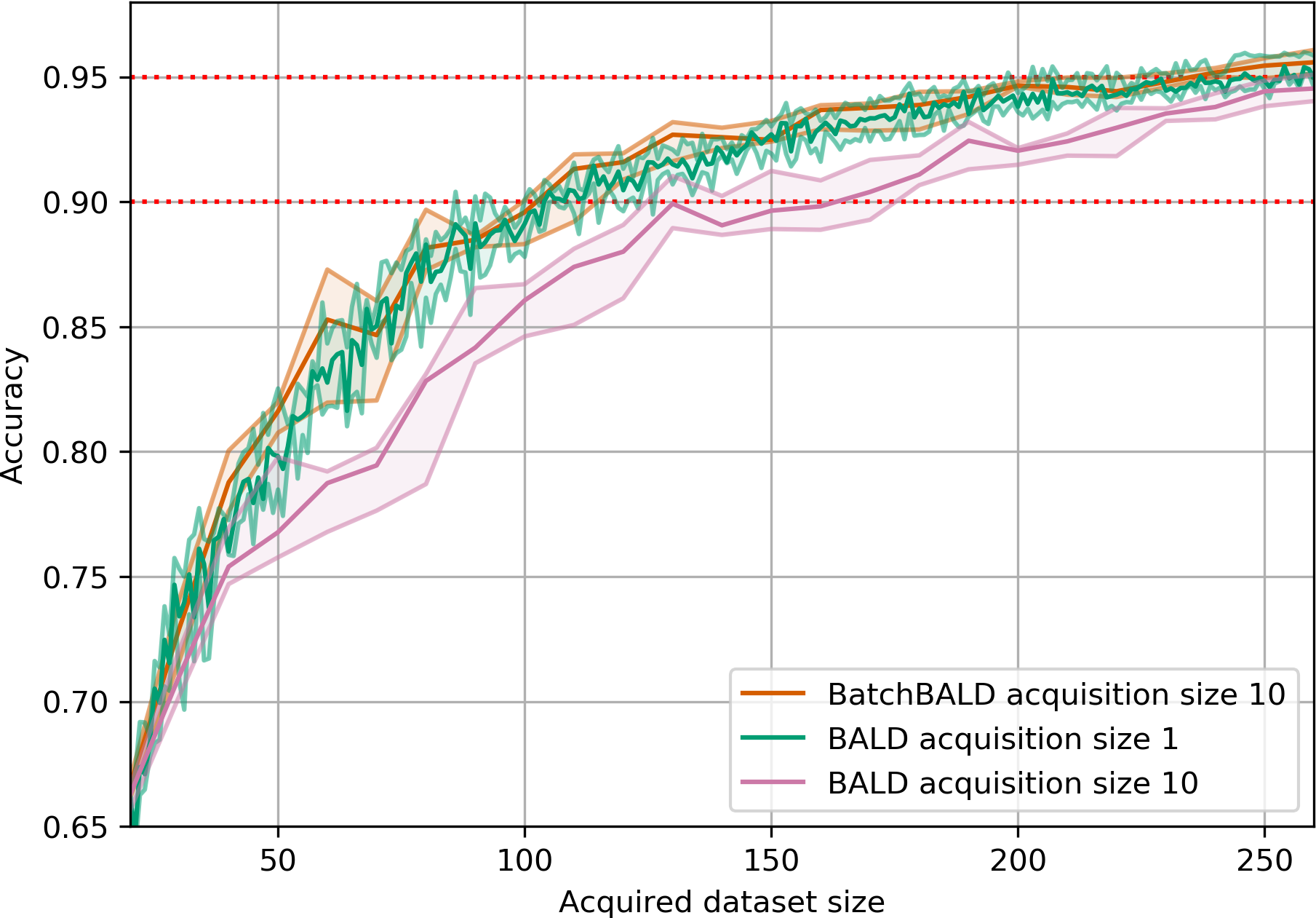
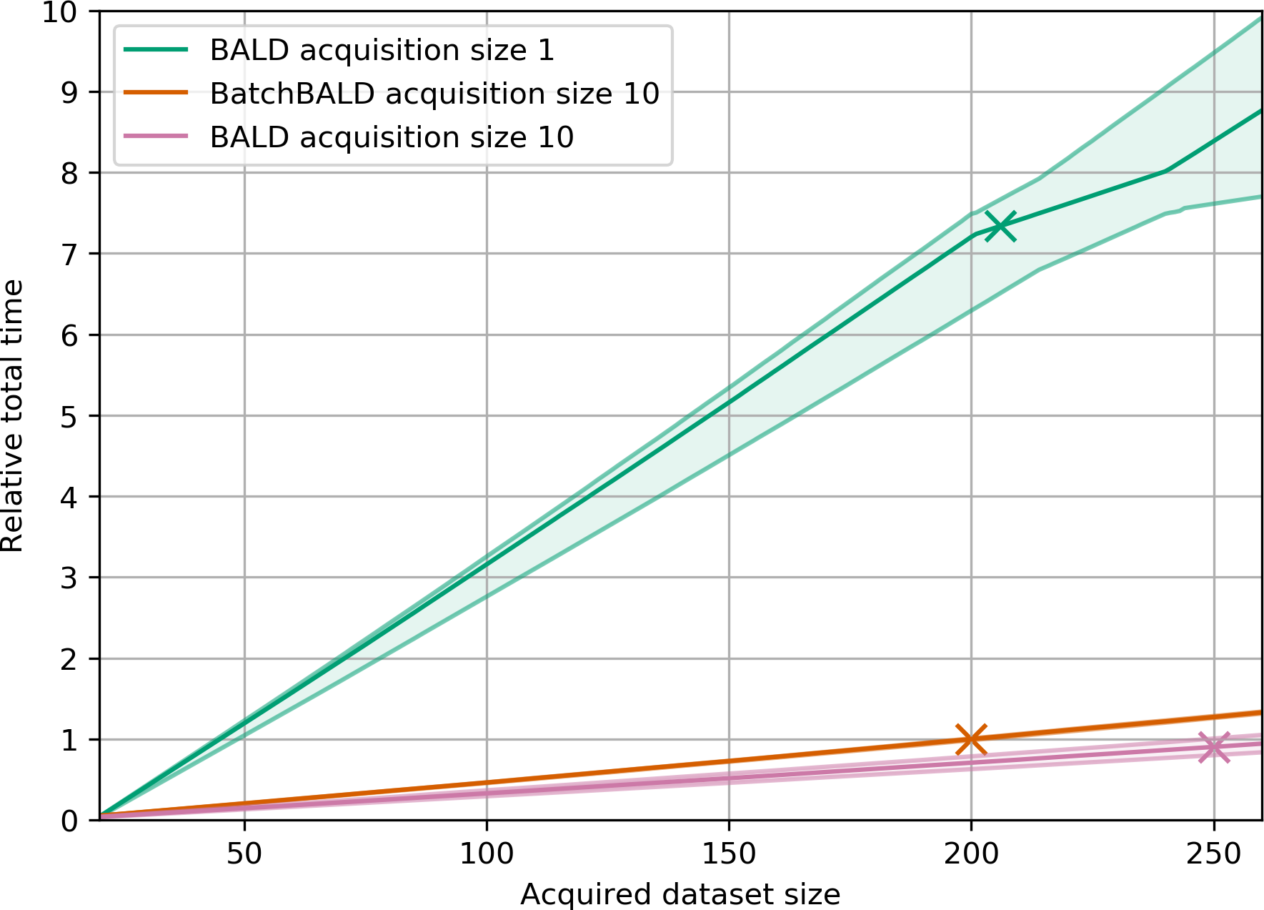
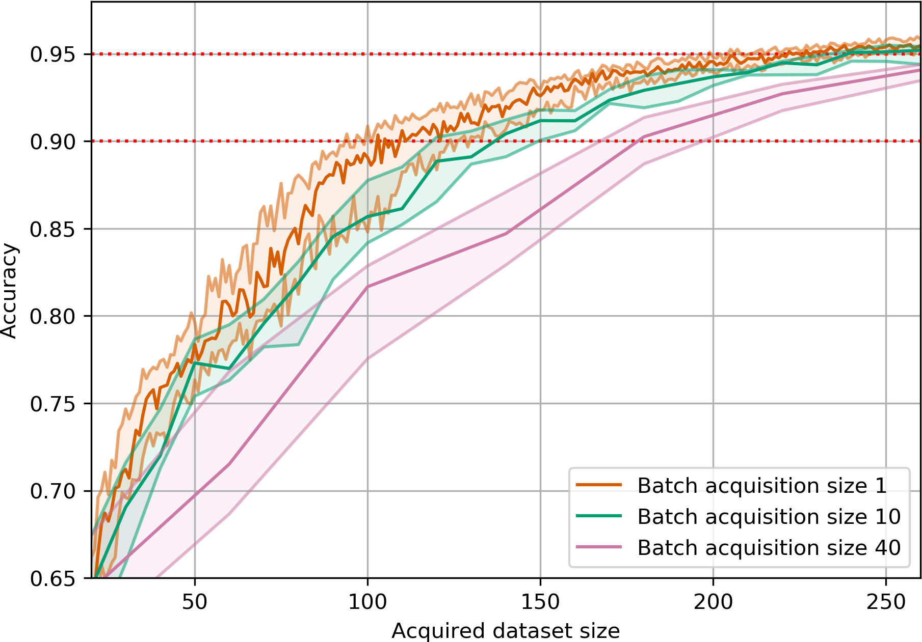
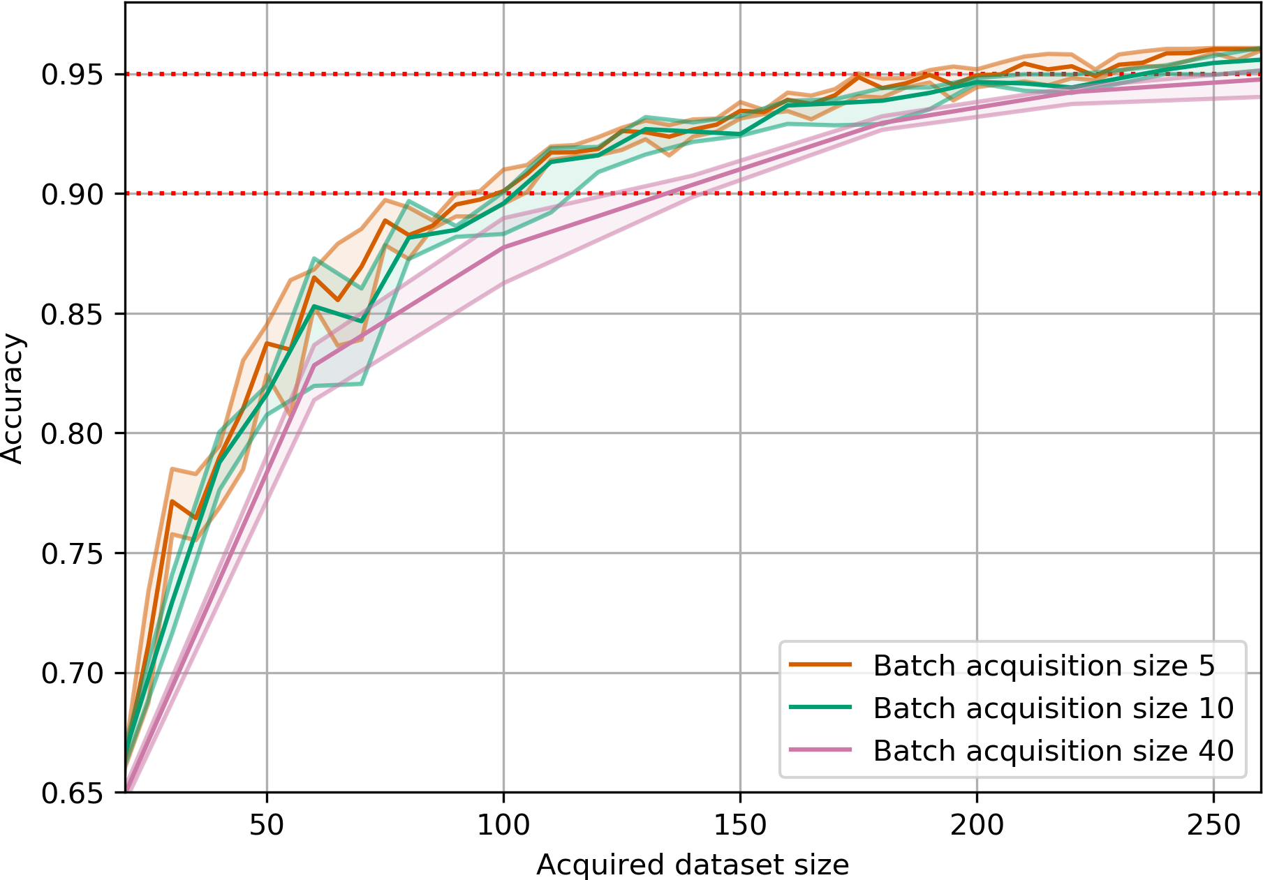
    return joint_entropies

Acquisition Size Ablation

EMNIST

EMNIST is a dataset of 28x28 grayscale images of handwritten digits and letters.

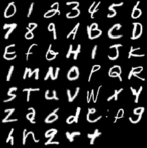
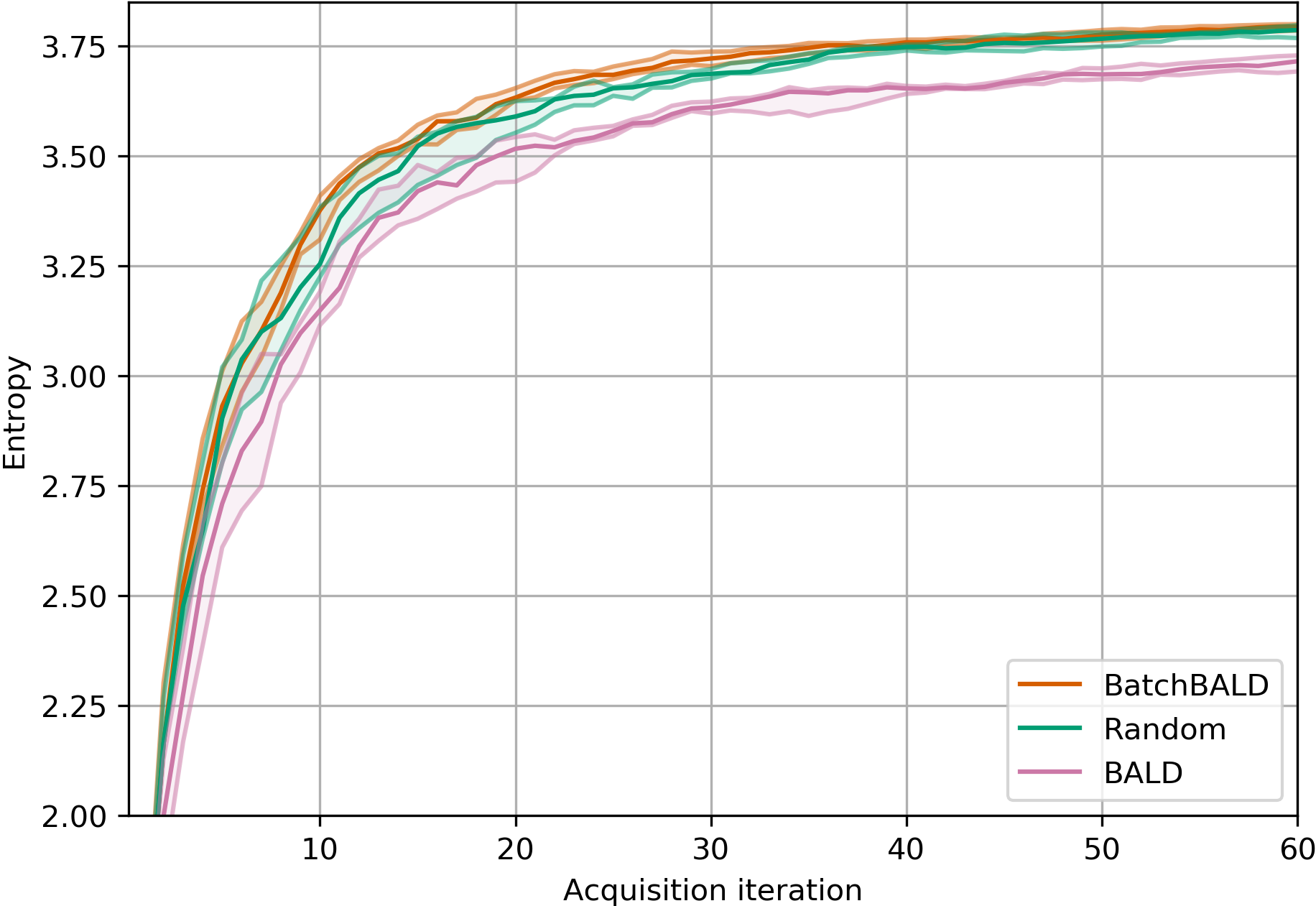
EMNIST Results

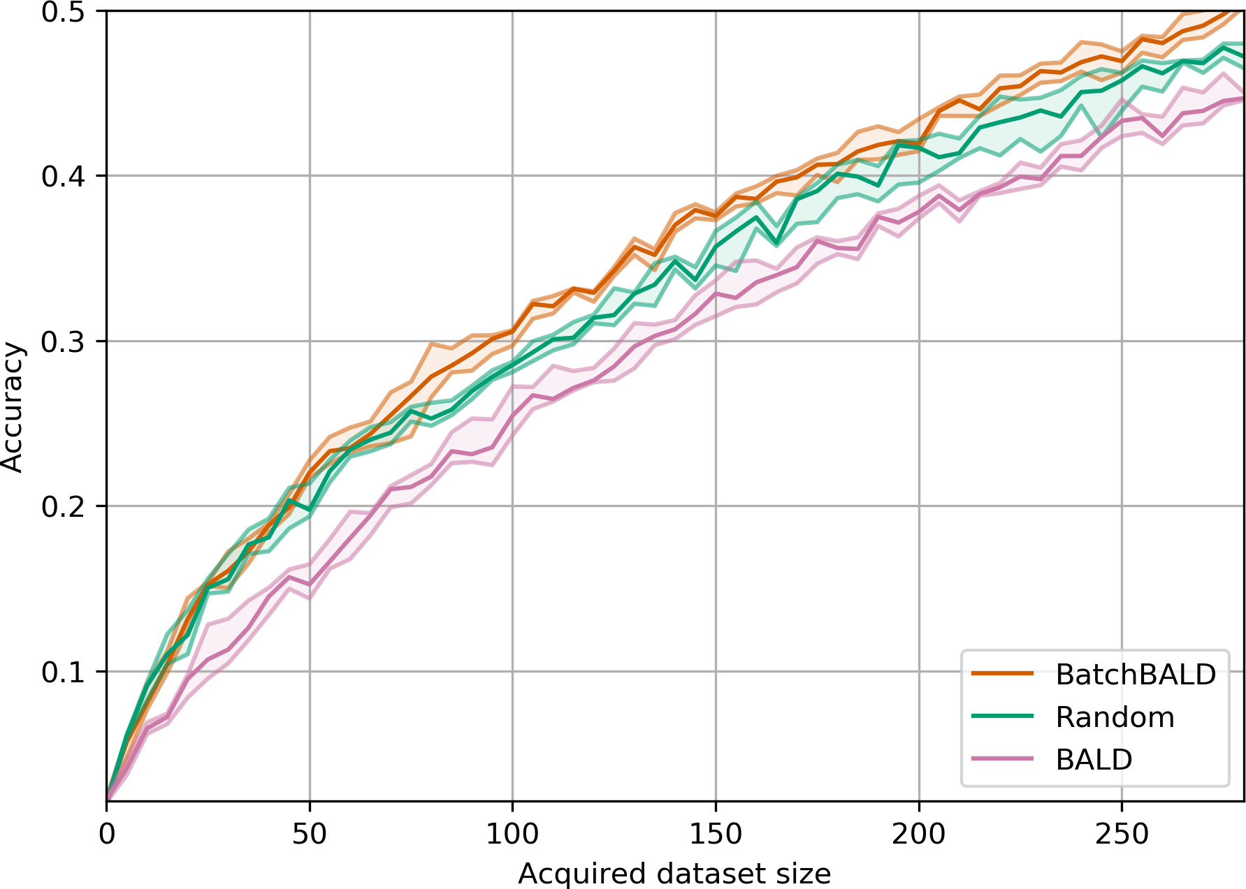
BatchBALD consistently outperforms both random acquisition and BALD while BALD is unable to beat random acquisition.

Acquired Label “Entropy”

BatchBALD steadily acquires a more diverse set of data points.

Summary

Naive batch acquisition can select redundant points
BatchBALD uses joint mutual information
Submodularity enables efficient subset selection
Practical implementation considerations matter

Stochastic Batch Acquisition

The Problem

Traditional batch acquisition methods can be computationally expensive (in seconds)

K Top-K BADGE BatchBALD

10 0.2 ± 0.0 9.2 ± 0.3 566.0 ± 17.4

100 0.2 ± 0.0 82.1 ± 2.5 5,363.6 ± 95.4

500 0.2 ± 0.0 409.3 ± 3.7 29,984.1 ± 598.7
BatchBALD scales poorly with batch size (limited to 5-10 points)
Top-k selection ignores interactions between points
Need a more efficient yet simple approach that maintains diversity

K	Top-K	BADGE	BatchBALD
10	0.2 ± 0.0	9.2 ± 0.3	566.0 ± 17.4
100	0.2 ± 0.0	82.1 ± 2.5	5,363.6 ± 95.4
500	0.2 ± 0.0	409.3 ± 3.7	29,984.1 ± 598.7

Key Insight

Acquisition scores change as new points are added to training set
1. For BatchBALD, the difference is:
  
  \[ \begin{aligned} &\MIof{\Y ; \W \given \x} - \MIof{\Y ; \W \given \x, \Y_{\text{train}}, \x_{\text{train}}} \\ &=\MIof{\Y; \Y_{\text{train}}; \W \given \x, \x_{\text{train}}} \\ &=\MIof{\Y; \Y_{\text{train}} \given \x, \x_{\text{train}}} - \MIof{\Y; \Y_{\text{train}} \given \W, \x, \x_{\text{train}}} \\ &=\MIof{\Y; \Y_{\text{train}} \given \x, \x_{\text{train}}} \ge 0. \end{aligned} \]
2. But if we don’t want to compute this?
Single-point scores act as noisy proxies for future acquisition value
Instead of deterministic top-k selection, use stochastic sampling
Sample according to score-based probability distribution

Noise Addition vs Sampling

We can add noise to the scores and take the top-K.

OR: we can sample from the score-based distribution directly.

This “duality” is similar to the Gumbel-Softmax trick.

Gumbel-Top-k Theorem

Theorem 4 For scores $s_i$, $i \in \{1, \ldots, n\}$, batch size $k \le n$, temperature parameter $\beta > 0$, and independent Gumbel noise $\epsilon_i \sim \text{Gumbel}(0,\beta^{-1})$:

\[ \arg \text{top}_k \{s_i + \epsilon_i\}_i \]

is equivalent to sampling $k$ items without replacement:

\[ \text{Categorical}\left(\frac{\exp(\beta \, s_i)}{\sum_j \exp(\beta \, s_j)}, i \in \{1, \ldots, n\}\right) \]

See also Kool, Hoof, and Welling (2019);Maddison, Tarlow, and Minka (2014); Gumbel (1954).

Key Implications

Provides theoretical justification for stochastic batch acquisition
Temperature $\beta$ controls exploration-exploitation trade-off:
- $\beta \to \infty$: deterministic top-k
- $\beta \to 0$: uniform random sampling

Tip

Origin: The Gumbel-Softmax trick allows us to backpropagate through sampling operations, making it useful for both inference and training.

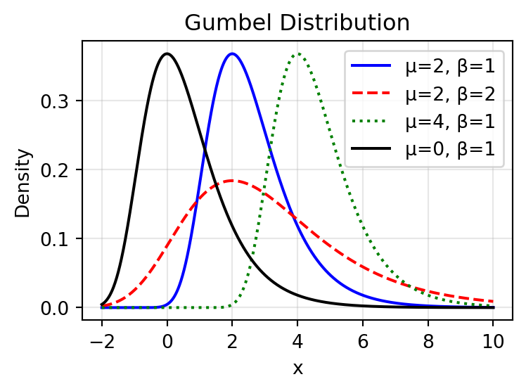
The Gumbel Distribution

The Gumbel distribution models the maximum of many random variables:

\[ F(x; \mu, \beta) = \exp\left(-\exp\left(-\frac{x-\mu}{\beta}\right)\right) \]

$\mu$ is the location parameter
$\beta$ is the scale parameter

Why Add Noise to Batch Selection?

The Problem with Top-K Selection

Assumption: Top-K assumes point scores are independent
Reality: Adding one point changes scores of all others
Key Insight: Most informative points cause biggest changes

Think About It…

What We Do:

Score all points
Pick top K at once

What Really Happens:

Score points
Add one point
Model updates
Scores change
Repeat…

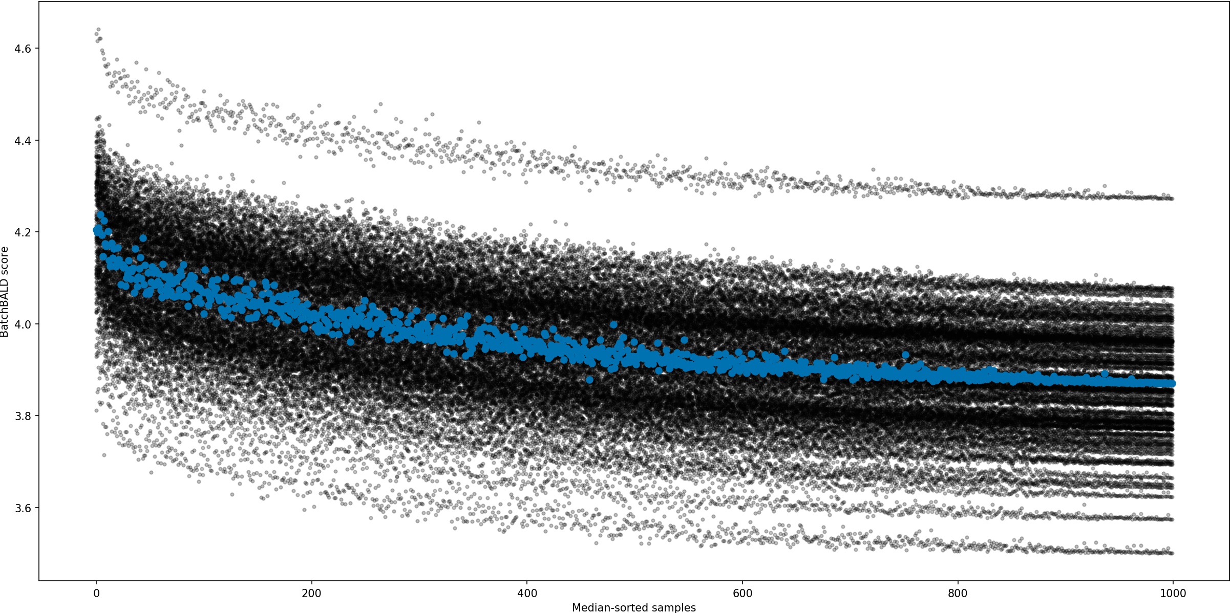
Score Correlation Over Time

Note

Scores become less correlated as we add points
Effect strongest for highest-scoring points
Larger batches = more uncertainty

Early acquisition scores are only a loose proxy for later scores. Specifically, the Spearman rank-correlation between acquisition scores on the first and n’th time-step falls with n. While top-acquisition incorrectly implicitly assumes the rank-correlation remains 1, stochastic acquisitions do not. BNN trained on MNIST at initial 20 points and 73% initial accuracy, score ranks over test set. — *Early acquisition scores are only a loose proxy for later scores.* Specifically, the Spearman rank-correlation between acquisition scores on the first and $n$’th time-step falls with $n$. While top-acquisition incorrectly implicitly assumes the rank-correlation remains $1$, stochastic acquisitions do not. BNN trained on MNIST at initial 20 points and 73% initial accuracy, score ranks over test set.

Details

Solution: Model the Uncertainty

Add Noise: Acknowledge score uncertainty
Sample Stochastically: Instead of deterministic top-K
Benefits:
- Natural diversity
- Matches reality better
- Simple & efficient

How It Works

import numpy as np
from scipy.special import softmax

def stochastic_batch_acquisition(pool_set, batch_size, model, temperature=1.0):
    # Score all points
    scores = []
    for x in pool_set:
        score = acquisition_function(x, model)
        scores.append(score)
    
    # Convert to probabilities
    probs = softmax(np.log(scores) / temperature)
    
    # Sample without replacement
    indices = np.random.choice(len(pool_set), size=batch_size, replace=False, p=probs)

    return indices

Benefits

Simple to implement ($\mathcal{O}(|P| + K \log |P|))$ complexity) for Gumbel noise w/ top-K
Naturally introduces diversity through stochastic sampling
Performs as well as or better than sophisticated methods
No hyperparameters to tune beyond temperature
Compatible with any acquisition scoring function

Results

Matches or outperforms BatchBALD and BADGE:

Repeated MNIST

EMNIST & MIO-TCD

Orders of magnitude faster computation

K	Top-K	Stochastic	BADGE	BatchBALD
10	0.2 ± 0.0	0.2 ± 0.0	9.2 ± 0.3	566.0 ± 17.4
100	0.2 ± 0.0	0.2 ± 0.0	82.1 ± 2.5	5,363.6 ± 95.4
500	0.2 ± 0.0	0.2 ± 0.0	409.3 ± 3.7	29,984.1 ± 598.7

Maintains performance with larger batch sizes
Avoids redundant selections common in top-k

Research Questions?

The strong performance of simple stochastic approaches raises serious questions about current complex batch acquisition methods:

Do they truly model point interactions effectively?
Are the underlying acquisition scores themselves reliable?
Is the additional computational complexity justified given similar performance?

$\implies$ Future work must develop more efficient methods that better capture batch dynamics while being tractable.

Appendix

References

Gumbel, Emil Julius. 1954. Statistical Theory of Extreme Values and Some Practical Applications: A Series of Lectures. Vol. 33. US Government Printing Office.

Kool, Wouter, Herke van Hoof, and Max Welling. 2019. “Stochastic Beams and Where to Find Them: The Gumbel-Top-k Trick for Sampling Sequences Without Replacement.” In Proceedings of the International Conference on Machine Learning (ICML), edited by Kamalika Chaudhuri and Ruslan Salakhutdinov, 97:3499–3508. Proceedings of Machine Learning Research. http://proceedings.mlr.press/v97/kool19a.html.

Maddison, Chris J., Daniel Tarlow, and Tom Minka. 2014. “A* Sampling.” In Advances in Neural Information Processing Systems, edited by Zoubin Ghahramani, Max Welling, Corinna Cortes, Neil D. Lawrence, and Kilian Q. Weinberger, 3086–94. https://proceedings.neurips.cc/paper/2014/hash/309fee4e541e51de2e41f21bebb342aa-Abstract.html.

Nemhauser, George L, Laurence A Wolsey, and Marshall L Fisher. 1978. “An Analysis of Approximations for Maximizing Submodular Set Functions—i.” Mathematical Programming 14 (1): 265–94.

Submodularity & Batch Acquisition

Why Batch Acquisition?

What You’ll Learn Today

Common Misconceptions

Batch Acquisition

Top-K Algorithm

Pseudocode

The Problem with Top-K

Redundancy Issue

Redundancy Issue

Simple Baseline

Batch Size Effect

Small Batch Size

Large Batch Size

Promise of Good Batch Acquisition

Saving Time and Labelling Cost

Information-Theoretic Perspective

BALD (≙ EIG)

Top-K Sum Equivalence

Top-K Intuition

Batch Intuition

I-Diagram \(\Rightarrow\) Information Quantity

Joint Mutual Information

Comparison

BALD

BatchBALD

Acquisition Function

Greedy Optimization

Guarantees

Submodularity

What is Submodularity?

Submodularity Visualization

Formal Definition

More Intuitive Definition?

Formal More Intuitive Definition

Proof of Equivalence

Simpler Definition

Proof

Summary

\(1 - \frac{1}{e}\) Optimality

Key Insights

Monotone Submodular Functions

Intuition

Questions

Submodular Non-/Monotone

Non-Submodular Non-Monotone

Optimality Proof

Statement

Greedy Algorithm

Goal

Key Concepts

Proof Sketch

Proof of \(\left(1 - \frac{1}{e}\right)\)-Optimality

Step 1: Bounding the Marginal Gain

Step 2: Recursive Inequality

Step 3: Unfolding the Recursion

Step 4: Limit Evaluation

Summary

Why?

Submodular BatchBALD

Marginal Gain

Proof (Last Step)

Proof: \(f(\emptyset) = 0\)

Proof: Monotone

Alternative:

Proof: Submodular

Summary

Revisiting the Greedy Algorithm

BatchBALD in Practice

Key Components

Results

Computing BatchBALD

Split

Computing the Joint

MC Sampling of \(\y_1, .., \y_n\)

Inconsistent MC Dropout

Easy Consistent Samples per Batch?

Consistent MC Dropout

Pseudo-Code

Efficient(?) Joint Entropy