Bayesian Neural Networks & Uncertainty
Comprehensive Overview
Why Uncertainty?
\[ \require{mathtools} \DeclareMathOperator{\opExpectation}{\mathbb{E}} \newcommand{\E}[2]{\opExpectation_{#1} \left [ #2 \right ]} \newcommand{\simpleE}[1]{\opExpectation_{#1}} \newcommand{\implicitE}[1]{\opExpectation \left [ #1 \right ]} \DeclareMathOperator{\opVar}{\mathrm{Var}} \newcommand{\Var}[2]{\opVar_{#1} \left [ #2 \right ]} \newcommand{\implicitVar}[1]{\opVar \left [ #1 \right ]} \newcommand\MidSymbol[1][]{% \:#1\:} \newcommand{\given}{\MidSymbol[\vert]} \DeclareMathOperator{\opmus}{\mu^*} \newcommand{\IMof}[1]{\opmus[#1]} \DeclareMathOperator{\opInformationContent}{H} \newcommand{\ICof}[1]{\opInformationContent[#1]} \newcommand{\xICof}[1]{\opInformationContent(#1)} \newcommand{\sicof}[1]{h(#1)} \DeclareMathOperator{\opEntropy}{H} \newcommand{\Hof}[1]{\opEntropy[#1]} \newcommand{\xHof}[1]{\opEntropy(#1)} \DeclareMathOperator{\opMI}{I} \newcommand{\MIof}[1]{\opMI[#1]} \DeclareMathOperator{\opTC}{TC} \newcommand{\TCof}[1]{\opTC[#1]} \newcommand{\CrossEntropy}[2]{\opEntropy(#1 \MidSymbol[\Vert] #2)} \DeclareMathOperator{\opKale}{D_\mathrm{KL}} \newcommand{\Kale}[2]{\opKale(#1 \MidSymbol[\Vert] #2)} \DeclareMathOperator{\opJSD}{D_\mathrm{JSD}} \newcommand{\JSD}[2]{\opJSD(#1 \MidSymbol[\Vert] #2)} \DeclareMathOperator{\opp}{p} \newcommand{\pof}[1]{\opp(#1)} \newcommand{\pcof}[2]{\opp_{#1}(#2)} \newcommand{\hpcof}[2]{\hat\opp_{#1}(#2)} \DeclareMathOperator{\opq}{q} \newcommand{\qof}[1]{\opq(#1)} \newcommand{\qcof}[2]{\opq_{#1}(#2)} \newcommand{\varHof}[2]{\opEntropy_{#1}[#2]} \newcommand{\xvarHof}[2]{\opEntropy_{#1}(#2)} \newcommand{\varMIof}[2]{\opMI_{#1}[#2]} \DeclareMathOperator{\opf}{f} \newcommand{\fof}[1]{\opf(#1)} \newcommand{\indep}{\perp\!\!\!\!\perp} \newcommand{\Y}{Y} \newcommand{\y}{y} \newcommand{\X}{\boldsymbol{X}} \newcommand{\x}{\boldsymbol{x}} \newcommand{\w}{\boldsymbol{\theta}} \newcommand{\W}{\boldsymbol{\Theta}} \newcommand{\wstar}{\boldsymbol{\theta^*}} \newcommand{\D}{\mathcal{D}} \newcommand{\HofHessian}[1]{\opEntropy''[#1]} \newcommand{\specialHofHessian}[2]{\opEntropy''_{#1}[#2]} \newcommand{\HofJacobian}[1]{\opEntropy'[#1]} \newcommand{\specialHofJacobian}[2]{\opEntropy'_{#1}[#2]} \newcommand{\indicator}[1]{\mathbb{1}\left[#1\right]} \]
The need for uncertainty in ML models stems from several critical factors.
Uncertainty for Active Learning
Uncertainty is a natural measure of informativeness in active learning:
- High uncertainty \(\rightarrow\) model is unsure \(\rightarrow\) learning opportunity
- Low uncertainty \(\rightarrow\) model is confident \(\rightarrow\) less to learn
Key Insight
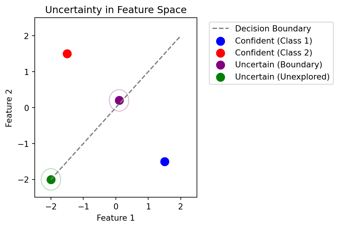
Uncertainty helps us find the decision boundary - where the model is most uncertain is where we need labels most.
Consider a binary classification problem:
- Points far from decision boundary: Model is confident \(\rightarrow\) low uncertainty
- Points near decision boundary: Model is uncertain \(\rightarrow\) high uncertainty
- Points in unexplored regions: Model should be uncertain \(\rightarrow\) high uncertainty
This motivates uncertainty sampling and its variants as acquisition functions.
Uncertainty about Uncertainty
Consider multiple valid hypotheses that explain our training data:
Key Insight
Even when a model expresses uncertainty through probabilities, there can be uncertainty about those probabilities, too. Different valid hypotheses (decision boundaries) that explain our training data can assign very different confidence values to the same point.
This highlights why we need:
- Any single decision boundary can be wrong and will be likely overconfident on some points.
- Methods to quantify uncertainty about uncertainty
- Ensembles or Bayesian averaging to capture hypothesis uncertainty
From Vision to Goals
What do we want from our deep learning models?
- Reliable uncertainty estimates (unknown unknowns)
- Calibrated confidence (known unknowns)
- Detection of out-of-distribution inputs (anomaly detection)
- Principled handling of uncertainty (theory)
- Detection of informative points (active learning)
Steps
- Foundations: Bayesian Statistics & Models
- Aleatoric vs Epistemic Uncertainty
- Information-theoretic Uncertainty
- Density-based Uncertainty
- Bayesian Deep Learning
- Approximation Methods
- Shallow Dive: Variational Inference
Last Years
Methods for BNNs:
- Mean Field VI (Blundell et al. 2015)
- MC Dropout (Gal and Ghahramani 2016)
- Deep Ensembles (Lakshminarayanan, Pritzel, and Blundell 2016)
- Laplace Approximation (Immer, Korzepa, and Bauer 2021)
What You Learn
- Foundations
- Connections between methods
- Trade-offs
- How to apply uncertainty methods
Bayesian Statistics
Three key principles that distinguish the Bayesian approach:
| Principle | Realization |
|---|---|
| Probability as degrees of belief | Everything is a R.V. |
| Parameters as random variables | Parameter distribution: \(\pof{\w}\) |
| Training data as evidence | Data likelihood: \(\pof{\D \given \w}\) |
| Learning is Bayesian inference | Update beliefs: \(\pof{\w \given \D}\) |
| Prediction via marginalization | Average over parameters: \(\E{\pof{\w}}{\pof{y \given x,\w}}\) |
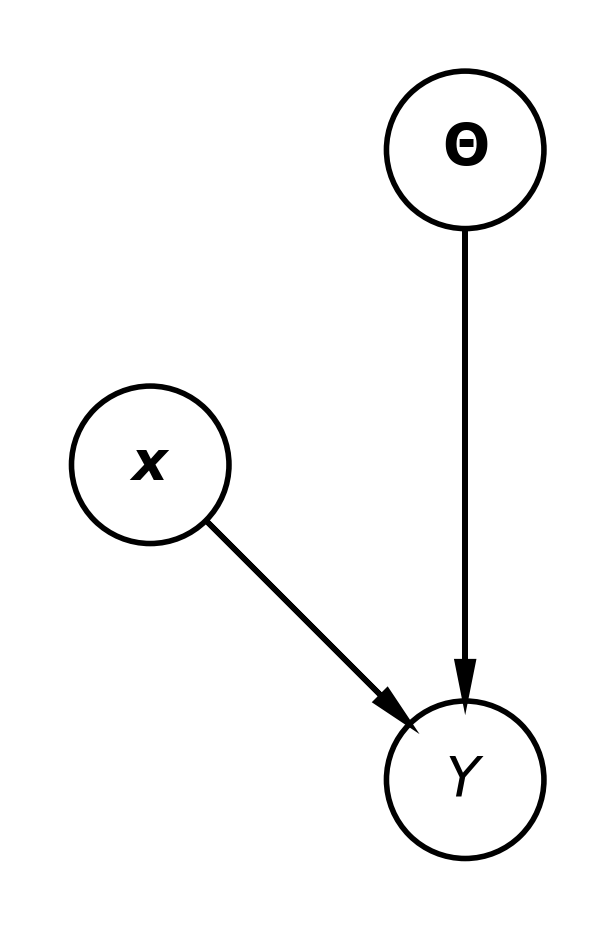
The Bayesian Model
Both the model parameters \(\w\) and the outputs \(\y\) for a given input \(\x\) are random variables. The joint distribution is defined as:
\[ \pof{\y, \w \given \x} = \pof{\y \given \x, \w} \pof{\w} \]
- Parameter distribution: \(\pof{\w}\): Captures our beliefs about the parameters.
- Data likelihood: \(\pof{\y \given \x, \w}\): Relates the inputs \(\x\) to outputs \(\y\) given parameters \(\w\).
Probability as Degrees of Belief
- Probabilities represent subjective beliefs
- Can assign probabilities to non-repeatable events
- Updates beliefs as new evidence arrives
- Prior knowledge can be formally incorporated
What it’s NOT: Frequentist
Probability as long-run frequency of events
- Requires repeatable experiments
- No formal way to include prior knowledge
- Only considers sampling distributions
Learning as Bayesian Inference
- Bayesian inference ≙ computing posterior \(\pof{\w \given \D}\)
- Combines prior knowledge with data
- Full distribution over parameters
- Automatic Occam’s razor effect
What it’s NOT
Point estimation (MLE/MAP):
- Single “best” parameter value
- No uncertainty quantification
- Can overfit without regularization
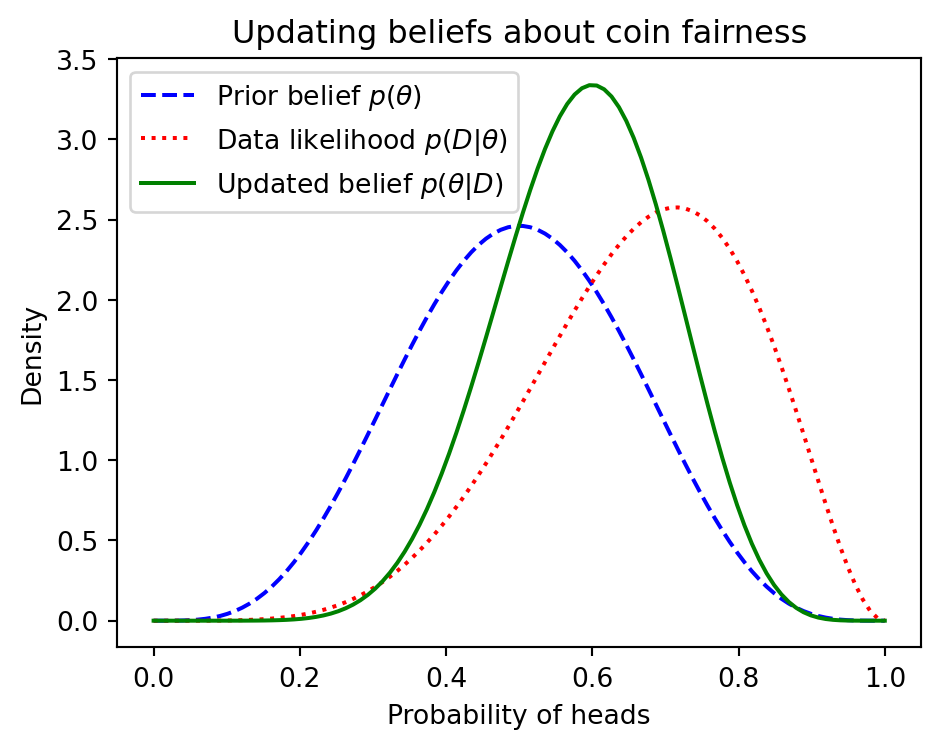
Bayesian Inference
\[ \underbrace{\pof{\w \given \D}}_{\text{posterior}} = \frac{\overbrace{\pof{\D \given \w}}^{\text{likelihood}} \; \overbrace{\pof{\w}}^{\text{prior}}}{\underbrace{\pof{\D}}_{\substack{\text{marginal likelihood} \\ \text{("evidence")}}}} \]
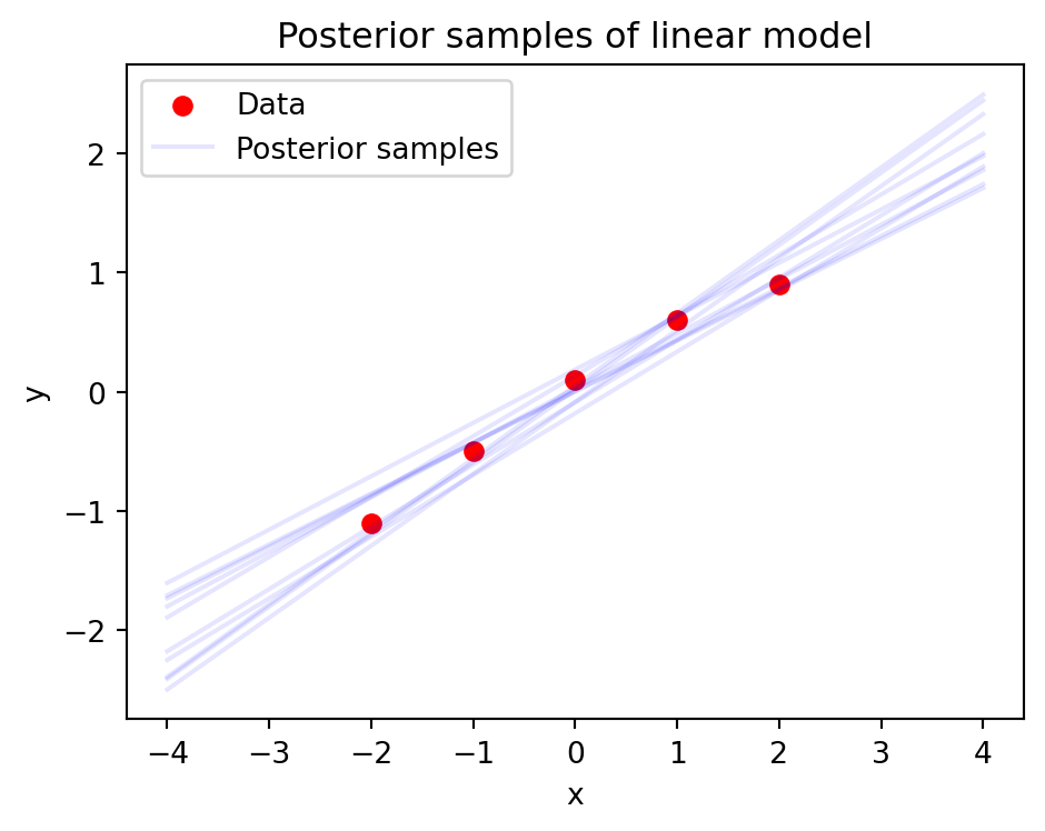
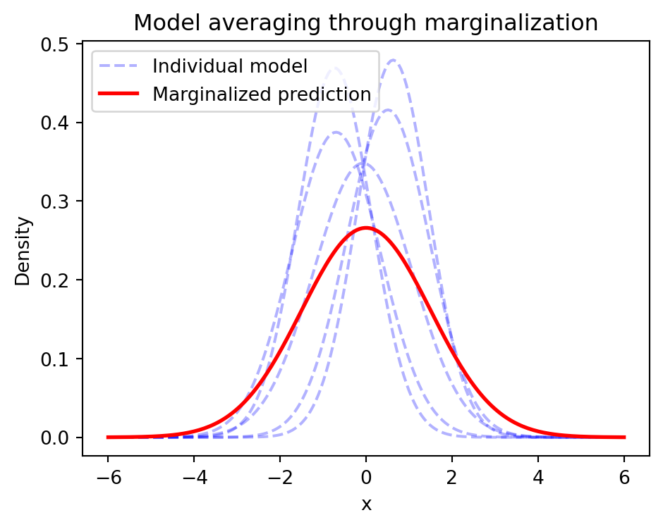
Prediction through Marginalization
- Average over all possible parameters
\[ \begin{aligned} \pof{y \given x,\D} &= \E{\pof{\w \given \D}}{\pof{y \given x, \w}} \\ &= \int \pof{y \given x,\w}\pof{\w \given \D}d\w \end{aligned} \]
- Naturally handles uncertainty
- Model averaging reduces overfitting
What it’s NOT
Plug-in prediction:
- Using single parameter estimate
- Ignores parameter uncertainty
- Can be overconfident
What Bayesian Stats is NOT
Frequentist Statistics
- Probability = long-run frequency
- Fixed parameters, random data
- Confidence intervals
- p-values and hypothesis tests
- Maximum likelihood estimation
Just Using Bayes’ Rule
- Bayes’ rule is just one tool
- Full Bayesian inference is more
- Not just about conditional probability
Merely Adding Priors
- Not just regularization
- Full uncertainty quantification
- Posterior predictive checks
- Model comparison
Only for Simple Models
- Scales to deep learning
- Practical approximations exist
- Active research area
- Modern computational tools
Summary
Parameter uncertainty: instead of \(\w^*\), use \(\pof{\w}\)
Start with prior beliefs \(\pof{\w}\)
Instead of optimizing the likelihood, update beliefs using data likelihood \(\pof{\D \given \w}\):
\[ \w^* = \arg \max_\w \pof{\D \given \w} \text{ vs. } \pof{\w \given \D} \]
Instead of point predictions, predict via marginalization:
\[ \pof{y \given x, \D} = \E{\pof{\w \given \D}}{\pof{y \given x,\w}} \]
Informativeness
- Informativeness measures how much information a given sample contains about the model parameters
- Active learning selects the most informative samples for labeling
How can we measure informativeness when we have a parameter distribution that captures our beliefs?
Reduction in Uncertainty
\(\equiv\) mutual information between model parameters and data:
\[ \MIof{\W; \Y \given \x} = \Hof{\W} - \Hof{\W \given \Y, \x}. \]
This is known as the Expected Information Gain (EIG).
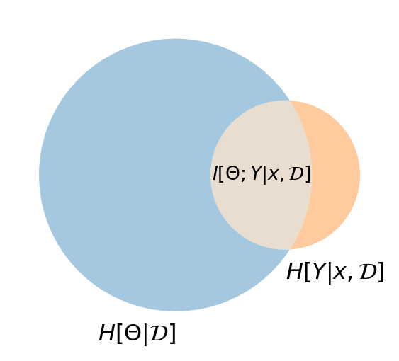
I-Diagram for the EIG

Expected Information Gain
Definition 1 The expected information gain is the mutual information between the model parameters \(\W\) and the prediction \(\Y\) given a new data point \(\x\) and already labeled data \(\D\):
\[ \MIof{\W; \Y \given \x, \D} = \Hof{\W \given \D} - \E{\pof{\y \given \x, \D}}{\Hof{\W \given \D, \y, \x}}. \]
Information Diagram
The overlapping region shows the mutual information between model parameters \(\W\) and predictions \(\Y\) given input \(\x\) and dataset \(\D\). This represents how much uncertainty about the predictions would be reduced if we knew the true parameters.
Historical Context: Expected Information Gain
The Expected Information Gain (EIG) has deep roots in experimental design:
Details
Historical Impact
These works established that selecting experiments to maximize information gain provides a principled approach to scientific discovery and machine learning.
Lindley (1956): “On a Measure of Information Provided by an Experiment”
- First formal treatment of information gain in Bayesian experiments
- Showed that Shannon entropy could quantify experimental value
- Introduced \(\MIof{\W; Y \given x}\) as design criterion
Box and Hill (1967): “Discrimination Between Mechanistic Models”
- Applied EIG to discriminate between competing chemical models
- Introduced sequential design of experiments
- Showed practical value in scientific discovery
MacKay (1992) : “Information-Based Objective Functions for Active Learning”
- Connected EIG to neural network active learning
- Showed equivalence to maximizing expected cross-entropy
- Laid groundwork for modern Bayesian active learning
BALD: A Practical Alternative
Bayesian Active Learning by Disagreement (BALD) provides a tractable approximation:
\[ \begin{aligned} \MIof{\W; \Y \given \x, \D} &= \MIof{\Y; \W \given \x, \D} \\ &= \Hof{\Y \given \x, \D} - \E{\pof{\w \given \D}}{\Hof{\Y \given \x, \w}}. \end{aligned} \]
Key Advantage
BALD requires only expectations over the model’s predictive distribution rather than explicit parameter uncertainty, making it more computationally feasible.
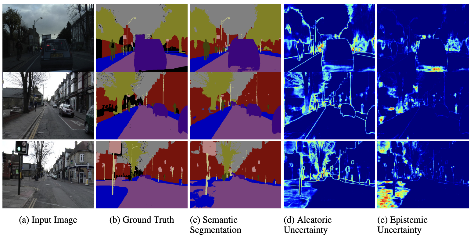
Aleatoric vs Epistemic Uncertainty
Two fundamental types of uncertainty:
- Aleatoric Uncertainty
- Inherent randomness in data
- Irreducible noise
- Present even with infinite data
- Epistemic Uncertainty
- Model’s lack of knowledge
- Reducible with more data
- High in regions without training data
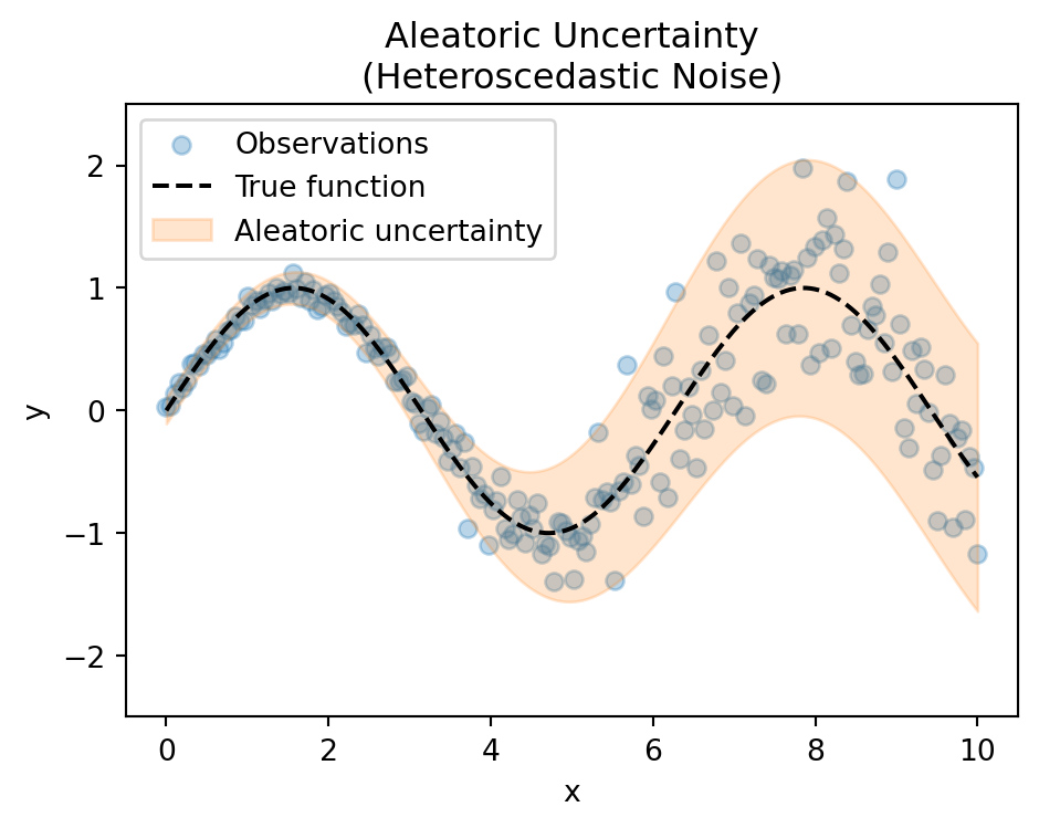
Aleatoric Uncertainty
- Inherent randomness in data
- Irreducible noise
- Present even with infinite data
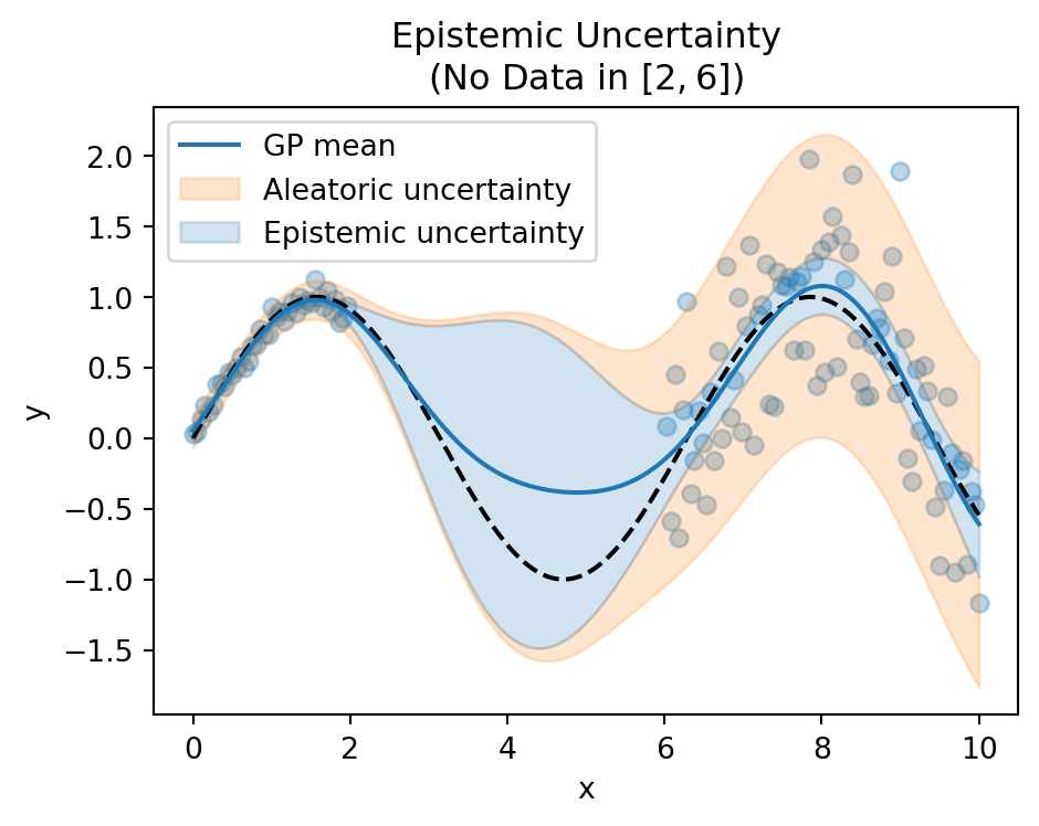
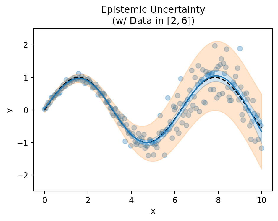
Epistemic Uncertainty
- Model’s lack of knowledge
- Reducible with more data
- High in regions without training data
Classification Example
Binary classification with overlapping regions and missing data
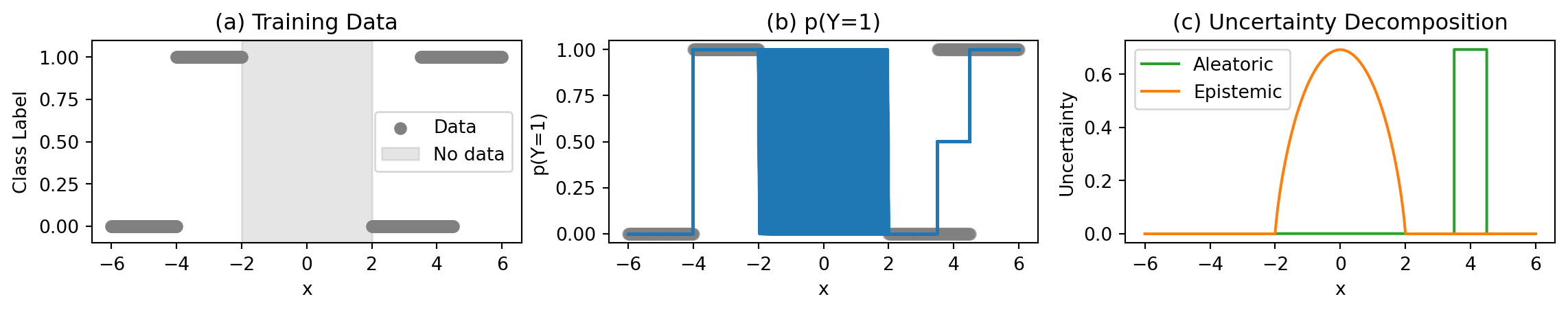
Key Regions in the Plots
Unambiguous Data Region:
- Confident predictions
- No aleatoric uncertainty
- No epistemic uncertainty
No Data Region (±2):
- Unknown predictions
- High epistemic uncertainty
- No aleatoric uncertainty
Ambiguous Data Regions $[3.5, 4.5]:
- Uncertain predictions
- High aleatoric uncertainty
- No epistemic uncertainty
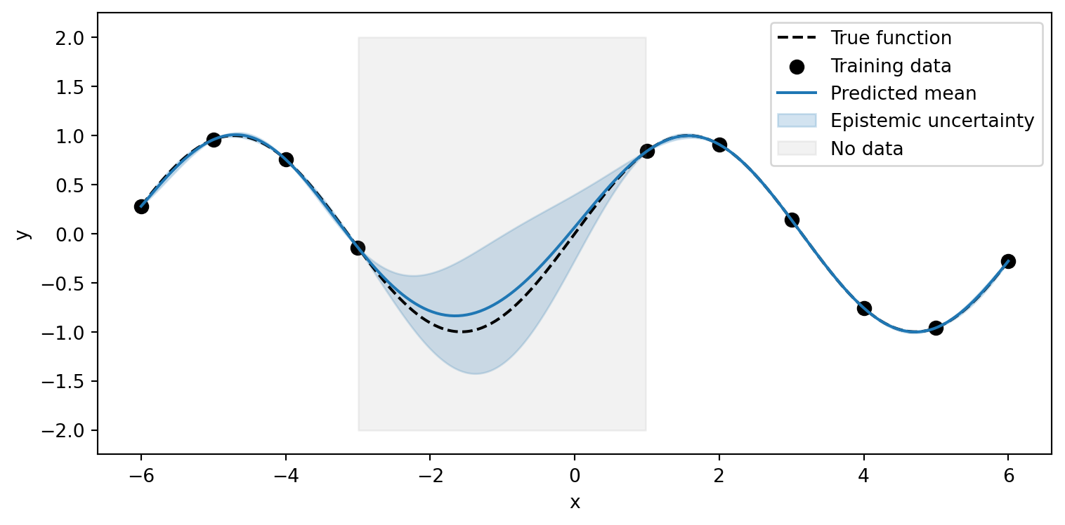
Uncertainty vs Generalization
Epistemic uncertainty and generalization are both shaped by our model’s inductive biases.
Key Insights
- Both manifest outside training data
- Inductive biases guide both uncertainty growth and generalization
- We can be correct while being uncertain (or not)
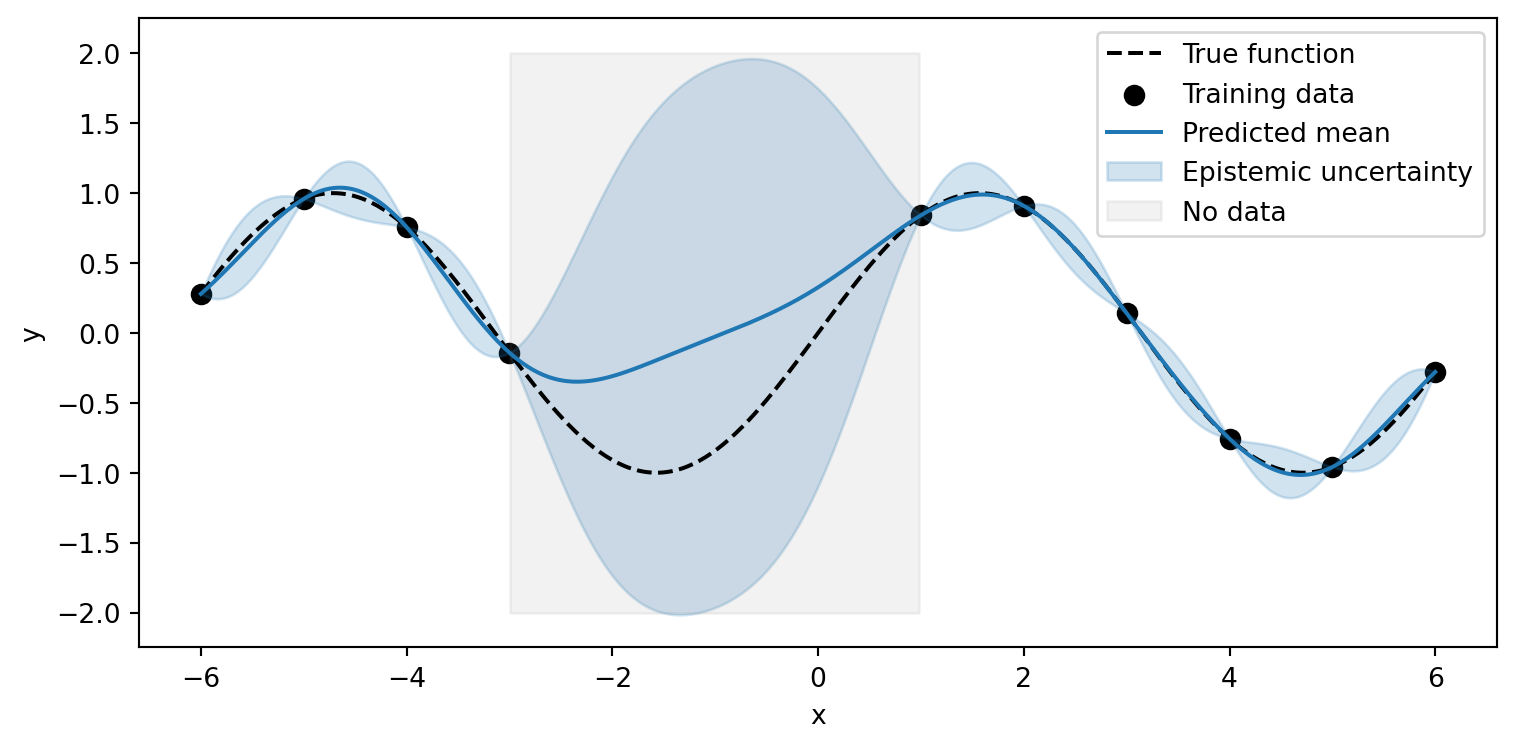
Uncertainty vs Generalization
Epistemic uncertainty and generalization are both shaped by our model’s inductive biases.
Key Insights
- Both manifest outside training data
- Inductive biases guide both uncertainty growth and generalization
- We can be correct while being uncertain (or not)
Key Differences
Aleatoric Uncertainty
- Data noise/randomness
- Cannot be reduced
- Often homoscedastic or heteroscedastic
- Present even with infinite data
Example: Measurement noise in sensors
Epistemic Uncertainty
- Model’s knowledge gaps
- Reducible with data
- High in sparse data regions
- Approaches zero with infinite data
Example: Predictions far from training data
Key Insight
Epistemic uncertainty decreases as we add more training data, while the true aleatoric uncertainty is independent of the model.
Information-Theoretic Uncertainty
Total Uncertainty Decomposition
Total uncertainty can be decomposed using information theory:
\[ \underbrace{\Hof{\Y \given \x}}_{\text{total uncertainty}} = \underbrace{\MIof{\Y; \W \given \x}}_{\text{epistemic}} + \underbrace{\Hof{Y \given \x, \W}}_{\text{aleatoric}} \]
Key Insight
This decomposition separates uncertainty into:
- What we could know (epistemic) - reducible with more data
- What we can’t know (aleatoric) - irreducible noise
BALD: Bayesian Active Learning by Disagreement
The mutual information term \(\MIof{Y; \W \given x}\) measures:
- Agreement between models (ensemble disagreement)
- Reduction in predictive uncertainty if we knew true parameters
- Uncertainty that could be reduced with more data
Classification Example
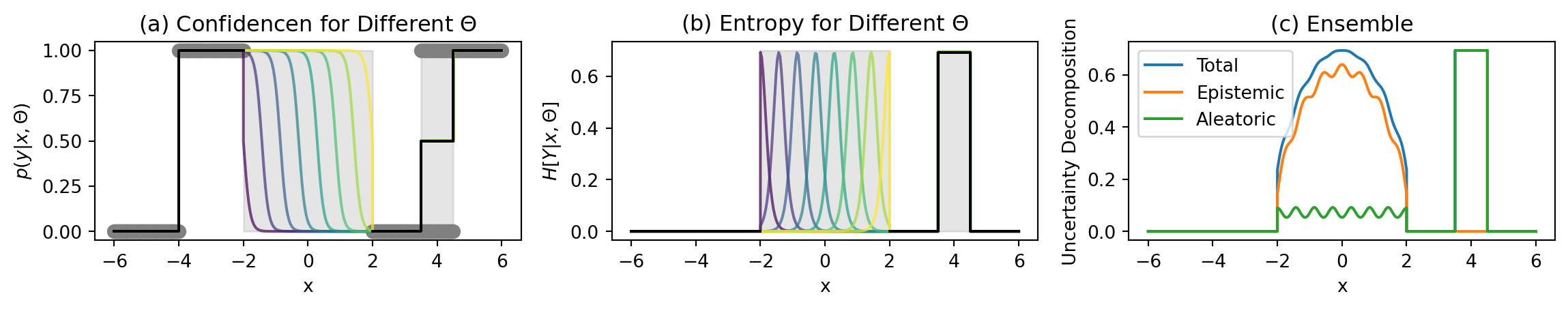
Key Regions
Unambiguous points (-6–-4):
- No uncertainty
- Confident predictions
No data region (-2–2):
- High predictive entropy (Total Uncertainty)
- High mutual information (Epistemic Uncertainty)
- Low softmax entropy (Aleatoric Uncertainty)
Ambiguous points points (3.5–4.5):
- High softmax entropy (Aleatoric Uncertainty)
- High predictive entropy (Total Uncertainty)
- Low mutual information (Epistemic Uncertainty)
Approximation Effect
Summary
\[ \underbrace{\Hof{\Y \given \x}}_{\text{total}} = \underbrace{\MIof{\Y; \W \given \x}}_{\text{epistemic}} + \underbrace{\E{\pof{\w \given \D}}{\Hof{\Y \given \x, \w}}}_{\text{aleatoric}} \]
- \(\Hof{\Y \given \x}\): Predictive entropy of averaged predictions
- What we observe in practice
- \(\MIof{\Y; \W \given \x}\): Mutual information between predictions and parameters
- Reducible through data collection
- High in regions without training data
- \(\E{\pof{\w \given \D}}{\Hof{\Y \given \x, \w}}\): Expected entropy under parameter distribution
- Irreducible noise in the data
- Present even with infinite data
Why Bayesian Model Average?
TL;DR: It’s the best we can do.
Details
Assume:
The model is well-specified: the true model is in our model class, so there are \(\w^{\text{true}}\) that generated the data.
Assume our beliefs \(\pof{\w}\) are rational and reflect the best we can do: otherwise, we would pick a different parameter distribution.
Then:
\[ \E{\pof{\w}}{\Kale{\pof{\Y \given \x, \w}}{\qof{\Y \given \x}}}, \]
captures how much worse any \(\qof{\y \given \x}\) is than the true (but unknown) model \(\pof{\y \given \x, \w^{\text{true}}}\) in expectation according to our beliefs \(\pof{\w}\).
We have:
\[ \begin{aligned} \E{\pof{\w}}{\Kale{\pof{\Y \given \x, \w}}{\qof{\Y \given \x}}} &= \E{\pof{\w}}{\CrossEntropy{\pof{\Y \given \x, \w}}{\qof{\Y \given \x}}} \\ &\phantom{=} - \E{\pof{\w}}{\xHof{\pof{\Y \given \x, \w}}} \\ &= \CrossEntropy{\E{\pof{\w}}{\pof{\Y \given \x, \w}}}{\qof{\Y \given \x}} \\ &\phantom{=} - \xHof{\pof{\Y \given \x, \W}} \\ &= \CrossEntropy{\pof{\Y \given \x}}{\qof{\Y \given \x}} \\ &\phantom{=} - \xHof{\pof{\Y \given \x, \W}} \\ &\ge \xHof{\pof{\Y \given \x}} - \xHof{\pof{\Y \given \x, \W}} \\ &= \MIof{\Y ; \W \given \x}. \end{aligned} \]
This shows that the Bayesian model average is the best we can do: it minimizes the expected prediction error according to our beliefs. We can’t do better than this.
We also see: the expected information gain/epistemic uncertainty is a lower bound on the expected loss divergence between the true model and our predictions.
BMA: Summary
- Best we can do: minimizes expected prediction error
- Lower bound on expected loss divergence
- Epistemic uncertainty is the (expected) gap to the (expected) truth
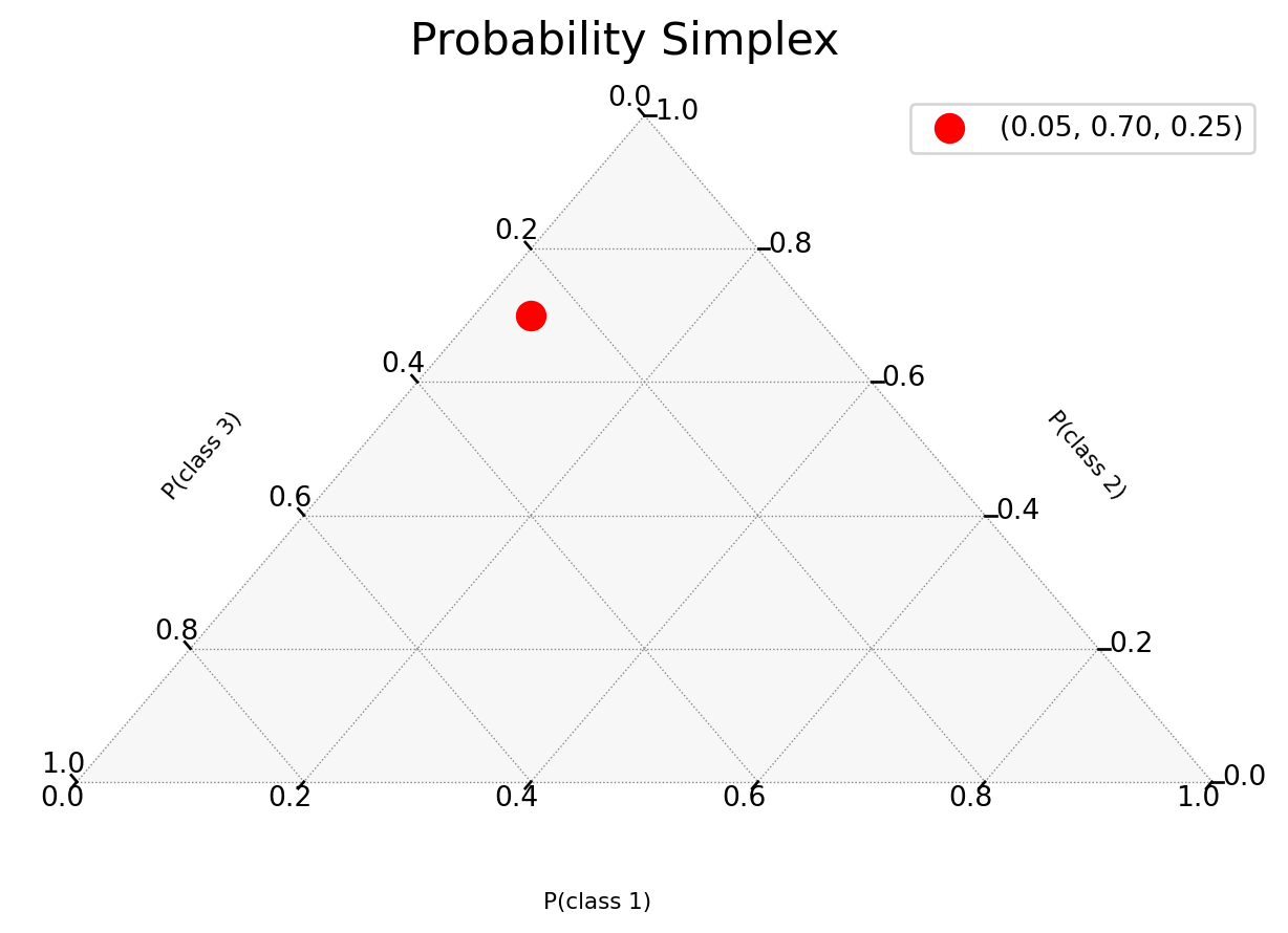
Probability Simplex
…or how to visualize predictions as points in the probability simplex.
Point Predictions vs Probability Vectors
A neural network’s softmax output may look like a probability distribution:
# Prediction for a single image
logits = model(x)
probs = softmax(logits)
>>> [0.05, 0.92, 0.03]  # Sums to 1
But this is still just a point estimate - a single point in the probability simplex:
\[ \Delta^{n-1} = \left\{ p \in \mathbb{R}^n : \sum_{i=1}^n p_i = 1, p_i \geq 0 \right\}. \]
Understanding the Probability Simplex
MC Samples in the Simplex
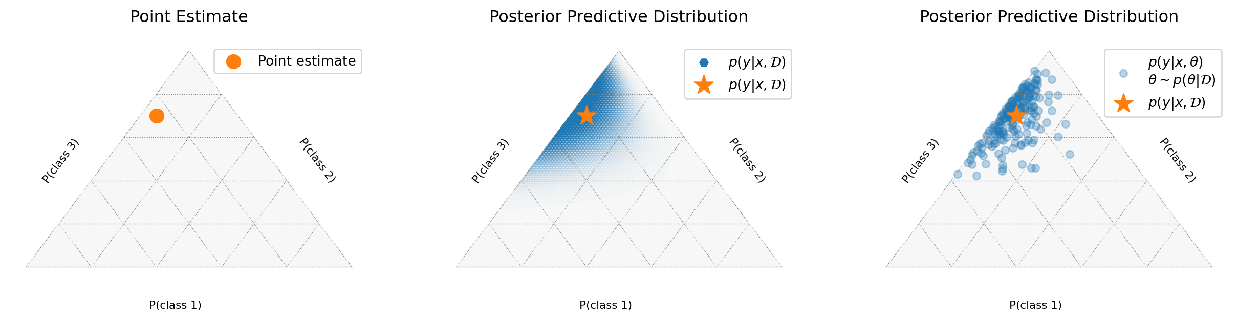
Visualizing Epistemic Uncertainty
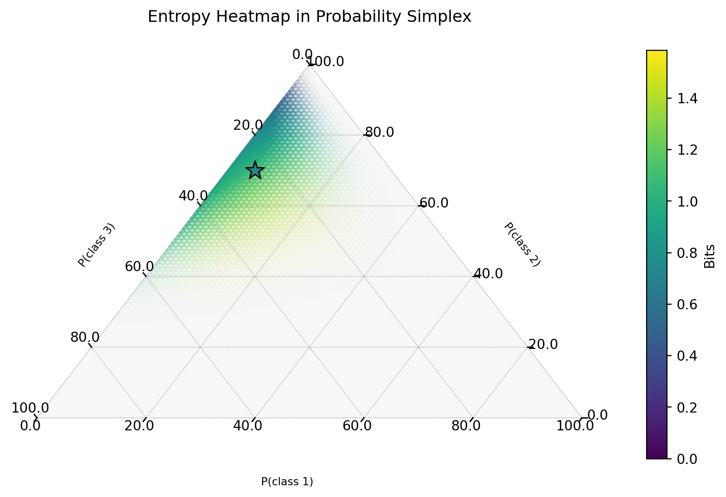
Visualizing Entropy Samples
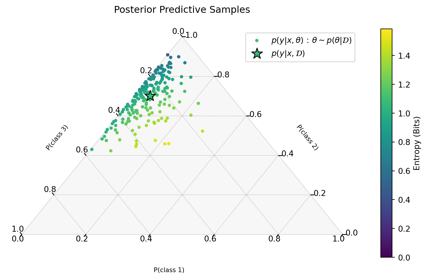
Interactive Plot
Asides
A few visualiations to understand the probability simplex, the concavity of the entropy, and the margin scores better…
Aside: Entropy Visualization
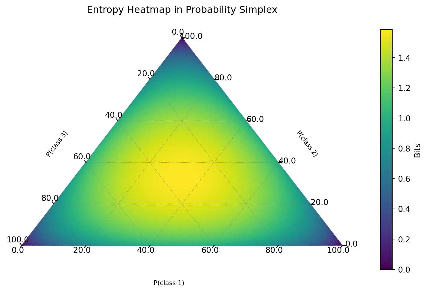
Interactive Plot
Aside: Margin Visualization
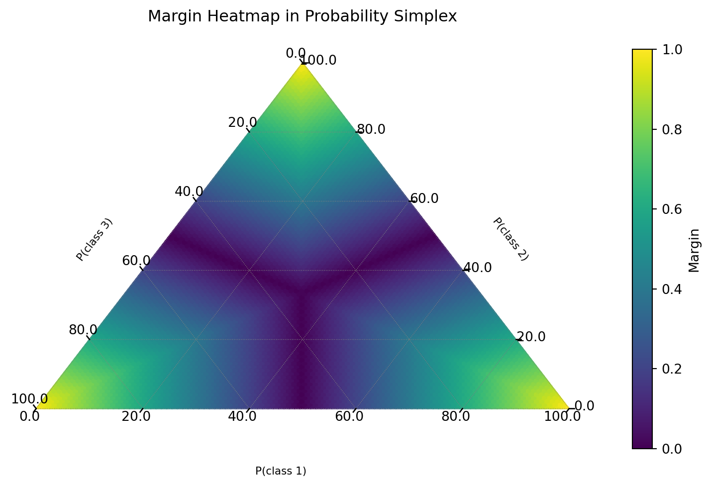
Interactive Plot
Comparison: Margin vs Entropy
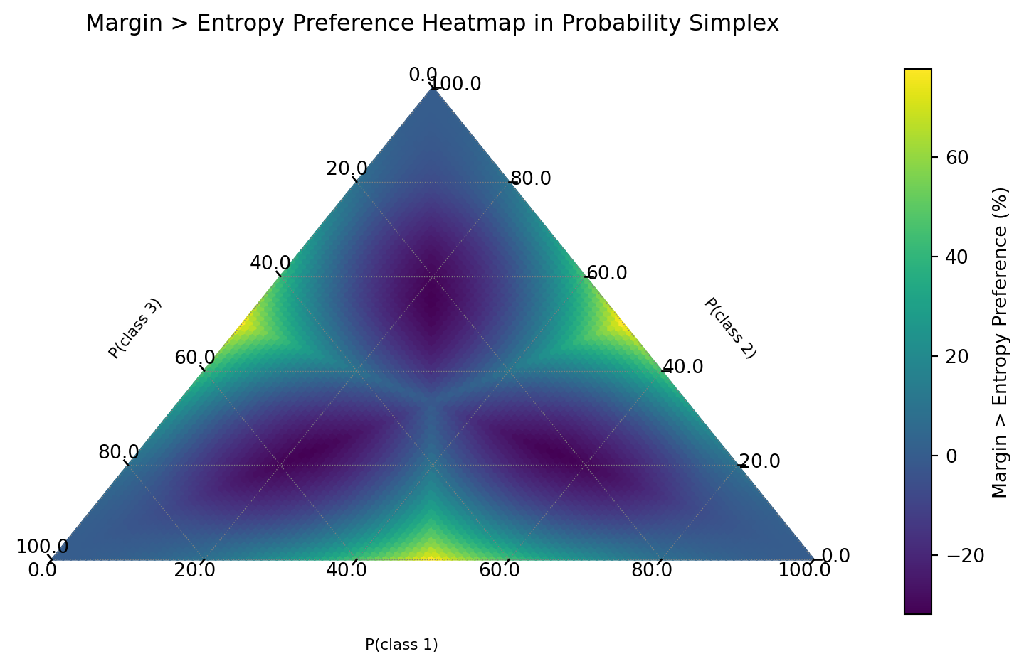
Interactive Plot
Density-based Uncertainty
Epistemic uncertainty ≙ reducible with more data
\(\overset{?}{\implies}\) use sample density \(\pof{x}\) to estimate uncertainty
But what about generalization to new inputs?
\[ \underbrace{X}_{\text{inputs}} \xrightarrow[\text{encoder}]{f(\cdot;\theta)} \underbrace{Z}_{\text{latents}} \xrightarrow[\text{classifier}]{\text{linear} + \text{softmax}} \underbrace{Y}_{\text{outputs}} \]
\(\overset{?}{\implies}\) use feature-space density \(\pof{f(x)}\) to estimate uncertainty?
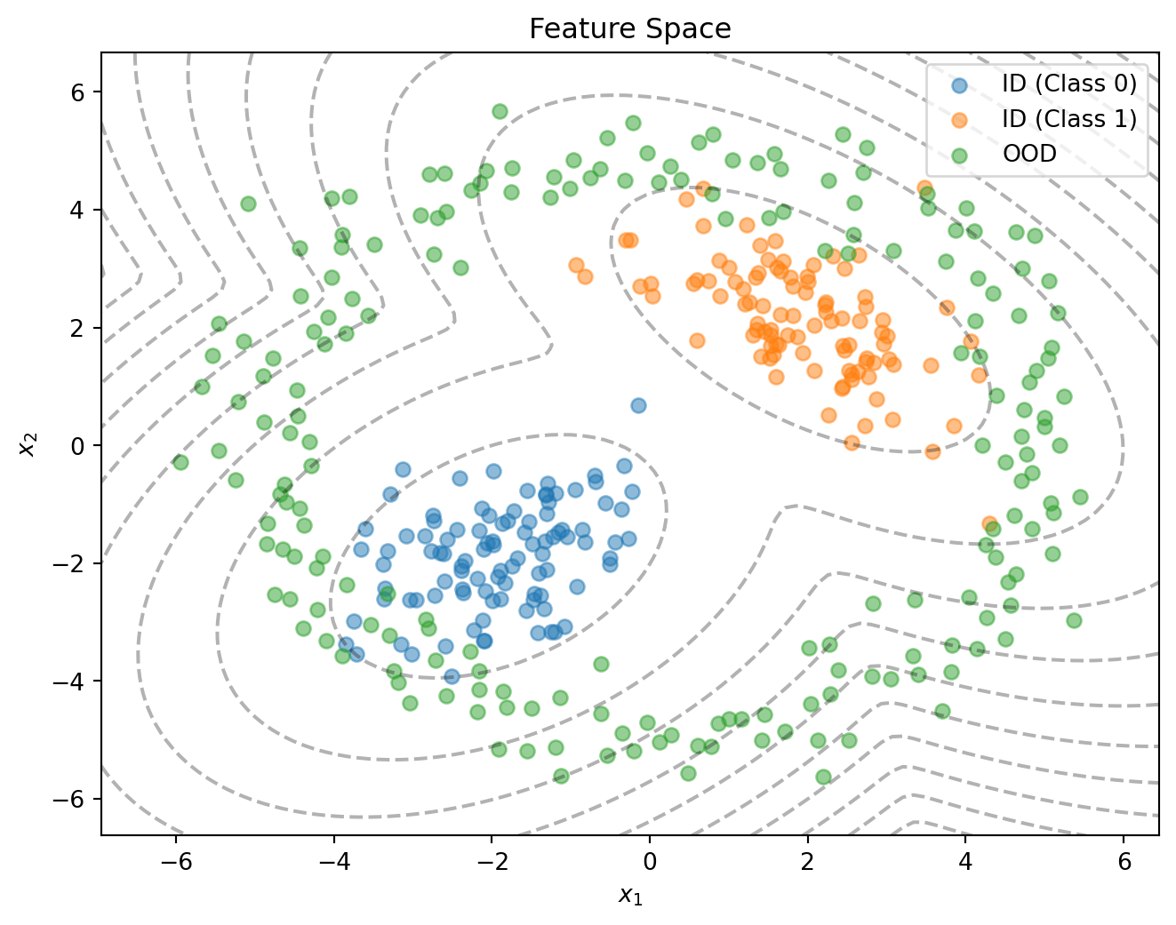
Key Idea
Density-based uncertainty leverages feature space density to estimate uncertainty:
- High density → Likely in-distribution
- Low density → Likely out-of-distribution
- No parameter distribution or sampling required!
Feature Space Density
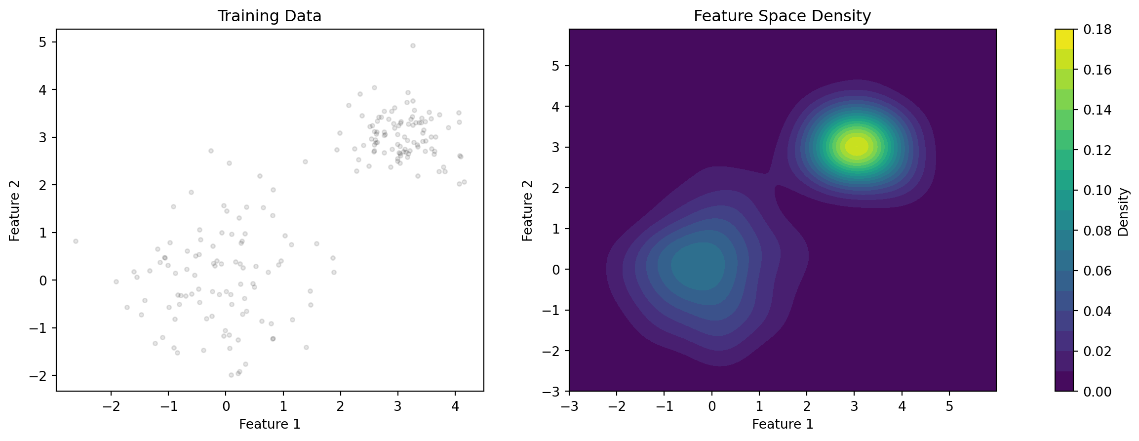
Advantages
Benefits:
- Single forward pass
- No sampling required
- Computationally efficient
- Natural OOD detection
Limitations:
- Requires density estimation
- Curse of dimensionality
- May miss class-specific uncertainty
Issues
- How do we estimate the density?
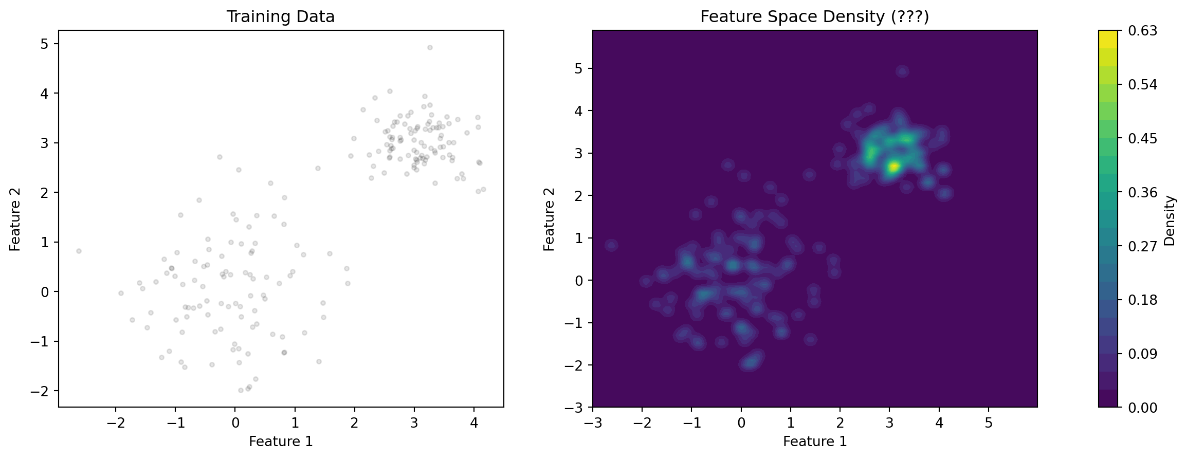
- How do take the decision boundaries for the classifier into account?
Deep Deterministic Uncertainty (DDU)
Key components:
- Feature extractor with spectral normalization
- Softmax classifier \(\implies\) Predictions + Aleatoric Uncertainty
- Class-conditional Gaussian density estimation \(\implies\) Epistemic Uncertainty
DDU Pseudocode
class DDU(nn.Module):
    def __init__(self):
        self.model = SpectralNormNet(classifier = SoftmaxClassifier())
        self.density_estimator = ClassConditionalGMM()
        self.density_ecdf = None

    def fit(self, X, y):
        self.model.fit(X, y)
        latents = self.model.encode(X)
        densities = self.density_estimator.fit(latents, y).score_samples(latents)
        self.density_ecdf = scipy.stats.ecdf(densities).cdf.evaluate

    def predict(self, X):
        latents = self.model.encode(X)
        density = self.density_estimator.score_samples(latents)
        density_quantile = self.density_ecdf(density)
        return self.model.classify(latents), density_quantile
ClassConditionalGMM
import numpy as np
import scipy.special

from dataclasses import dataclass, field
from sklearn.mixture import GaussianMixture


@dataclass
class ClassConditionalGMM:
    gmms: list[GaussianMixture] = field(default_factory=list)
    class_priors: list[float] = field(default_factory=list)
    classes: list[int] = field(default_factory=list)
    counts: list[int] = field(default_factory=list)

    def fit(self, X, y, seed=42):
        """Fit the class-conditional GMMs to the data."""
        self.classes, self.counts = np.unique(y, return_counts=True)
        total_samples = len(y)

        for c, count in zip(self.classes, self.counts):
            X_c = X[y == c]
            gmm = GaussianMixture(n_components=1, random_state=seed)
            gmm.fit(X_c)
            self.gmms.append(gmm)
            self.class_priors.append(count / total_samples)

        return self

    def score_samples(self, X):
        """Compute the log-density for each sample in X."""
        log_class_densities = []
        for gmm, prior in zip(self.gmms, self.class_priors):
            log_class_density = gmm.score_samples(X)
            log_class_densities.append(log_class_density + np.log(prior))
        log_densities = scipy.special.logsumexp(log_class_densities, axis=0)

return log_densitiesClassConditionalGMM: Example
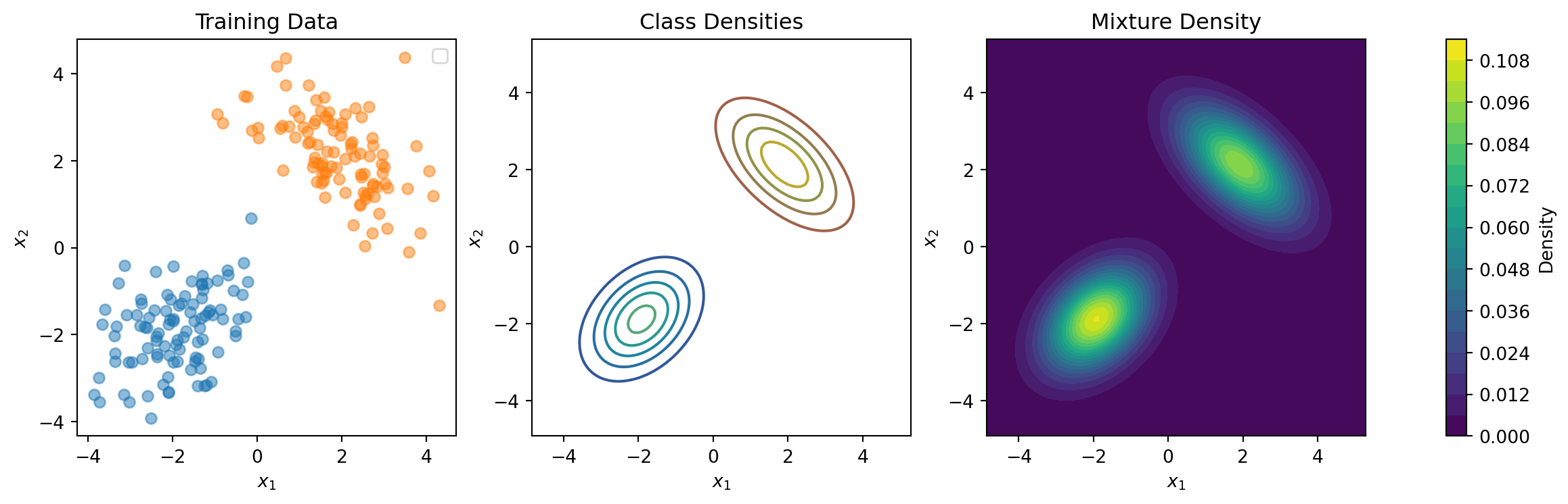
SimpleDDU (no features)
import matplotlib.pyplot as plt
from sklearn.metrics import roc_curve, auc
from sklearn.linear_model import LogisticRegression

class SimpleDDU:
    def __init__(self):
        self.classifier = LogisticRegression()
        self.density_estimator = ClassConditionalGMM()
        self.density_ecdf = None

    def fit(self, X, y):
        self.classifier.fit(X, y)
        densities = self.density_estimator.fit(X, y).score_samples(X)
        self.density_ecdf = scipy.stats.ecdf(densities).cdf.evaluate
        return self

    def predict(self, X):
        class_probs = self.classifier.predict_proba(X)
        density = self.density_estimator.score_samples(X)
        density_quantile = self.density_ecdf(density)
return class_probs, density_quantileSimpleDDU: Example
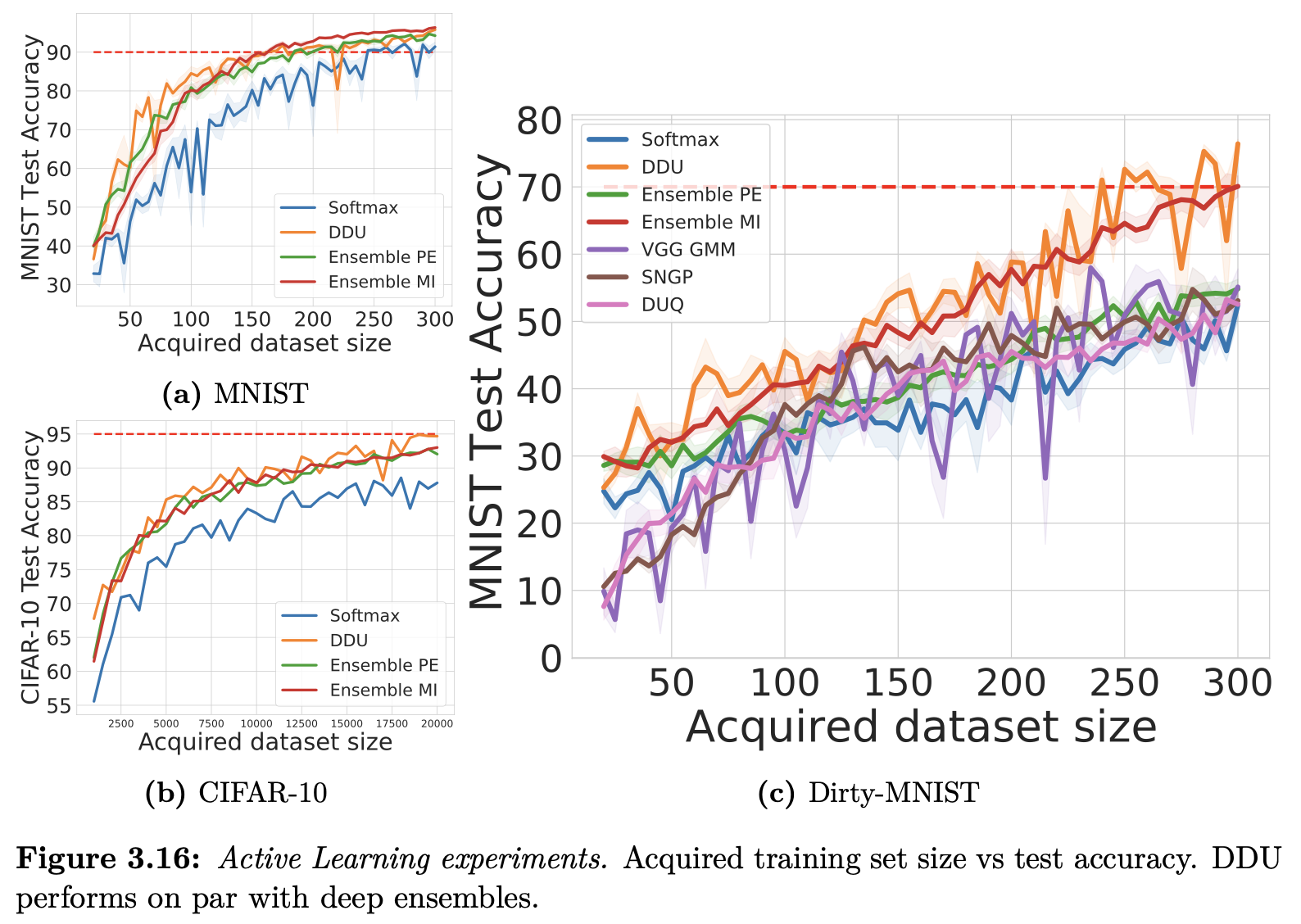
SimpleDDU: Results

DDU Paper Results
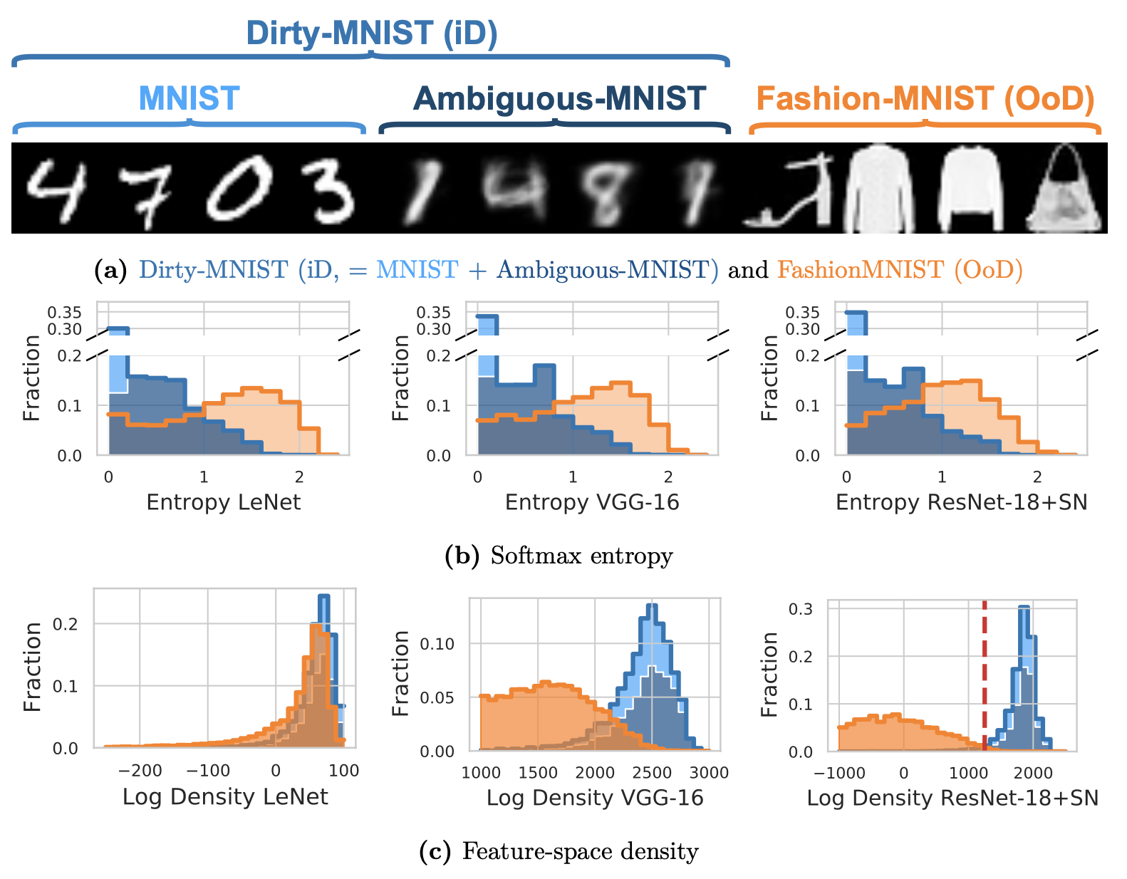
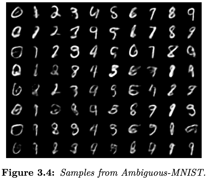
Dirty-MNIST
Density ≙ Epistemic Uncertainty
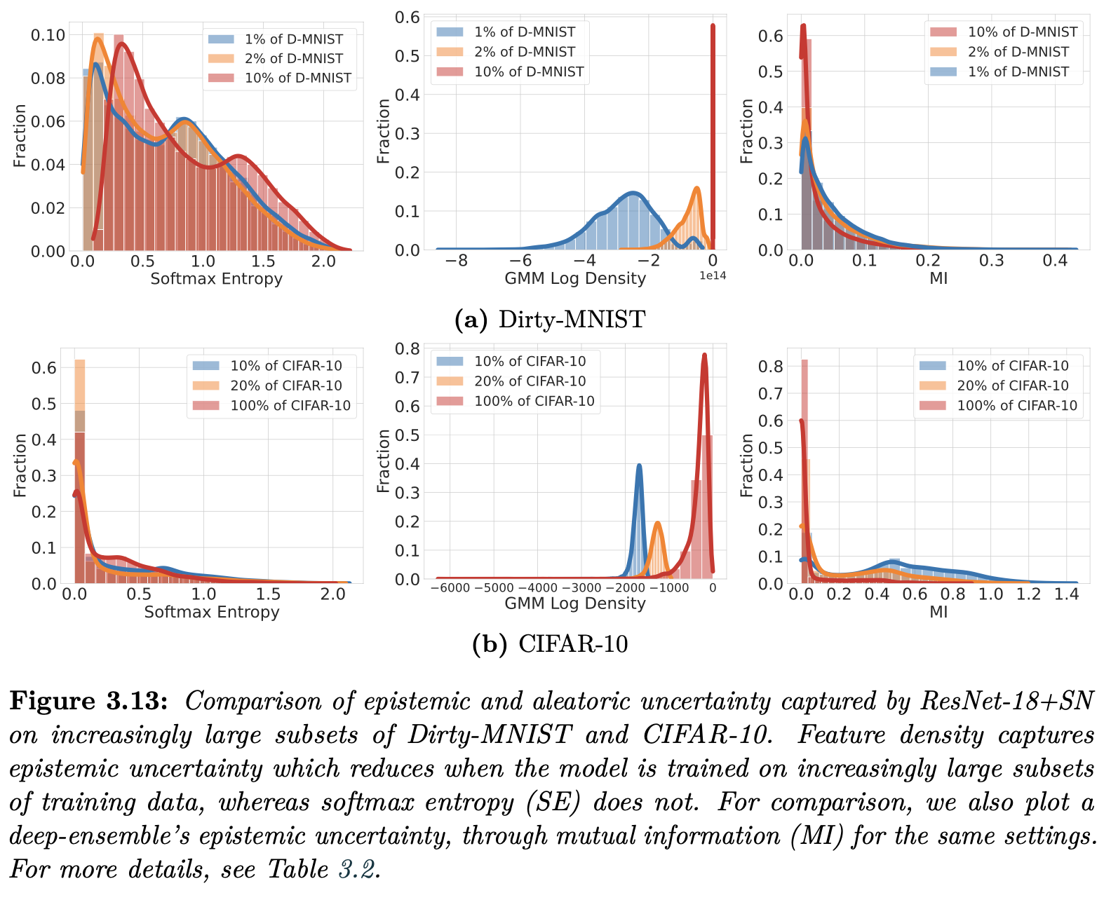
Density for Active Learning
Summary
Density-based uncertainty:
- Uses feature space density
- Single forward pass
- Natural OOD detection
- Computationally efficient
Key Insight
Combining density estimation with deep learning provides efficient uncertainty estimation without sampling!
OoD Detection vs AL
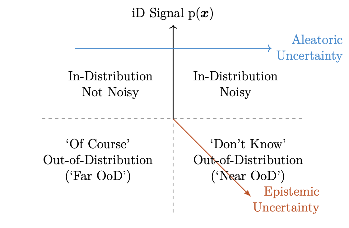
Key Distinctions
OOD detection and active learning approach uncertainty from complementary perspectives:
- OOD Detection prioritizes identifying samples that deviate from the training signal \(p(\mathbf{x})\)
- Primary goal: Flag anomalous inputs
- Less concerned with model’s epistemic uncertainty
- Focuses on binary decision: in or out of distribution?
- Active Learning prioritizes epistemic uncertainty
- Primary goal: Find informative samples to improve model
- Seeks regions where model is uncertain but learnable
- Often most valuable samples lie at distribution boundaries
Key insight: While OOD detection asks “Is this sample valid?”, active learning asks “What can we learn from this sample?”
Important
DDU works for AL because DDU’s experimental setup ensures that OoD detection and epistemic uncertainty are well-aligned (e.g., no far OoD data!).
Bayesian
Deep
Learning
The Ideal
The Bayesian ideal is to maintain a full posterior distribution over model parameters:
\[ \pof{\w \given \D} \]
This would allow us to:
- Make predictions with uncertainty quantification
- Automatically handle overfitting through marginalization
- Get principled uncertainty estimates
BUT…
Exact Bayesian inference is intractable for modern neural networks:
- High dimensionality (millions of parameters)
- Non-conjugate likelihoods
- Computational cost
Details
We cannot compute a density easily:
\[ \pof{\w \given \D} = \frac{\pof{\D \given \w} \pof{\w}}{\pof{\D}}, \]
requires \(\pof{\D} = \E{\pof{\w}}{\pof{\D \given \w}}\), which is intractable.
We cannot easily draw samples from the posterior either:
\[ \w \sim \pof{\w \given \D}. \]
Doing so requires MCMC or similar methods, which are computationally expensive and slow.
This leads us to approximations…
The Approximations
- Variational Inference
- Mean Field Approximation
- Monte Carlo Dropout
- Laplace Approximation
Variational Inference
“The one to rule them all.”
—Andreas Kirsch, 2024/12/04
Goal
- We have a complex posterior distribution \(\pof{\w \given \D}\)
- We want to approximate it with a variational distribution \(\qof{\w}\)
How can we do that?
Optimization Problem
\[ \min_{\qof{\w}} \Kale{\qof{\W}}{\pof{\W \given \D}} \searrow 0. \]
Variational Bayes
Variational Inference (VI) is a method for approximating the posterior distribution \(\pof{\w \given \D}\) with a variational distribution \(\qof{\w}\).
When we use VI for the Bayesian posterior, we call it Variational Bayes (VB).
\[ \qcof{*}{\w} \in \arg \min_{\qof{\w}} \Kale{\qof{\W}}{\pof{\W \given \D}}. \]
How does this help us?
- We can rewrite the KL divergence in closed form and make it tractable by dropping \(\pof{\D}\).
- We can optimize the KL divergence using gradient descent to find a good \(\qof{\w}\).
- We usually parameterize \(\qof{\w}\) with parameters \(\psi\), that is, we have \(\qcof{\psi}{\w}\) and optimize over \(\psi\).
Discovering the Evidence Bound
Also known as the Evidence Lower Bound (ELBO) when using probabilities.
\[ \begin{aligned} &\Kale{\qof{\W}}{\pof{\W \given \D}} = \CrossEntropy{\qof{\W}}{\pof{\W \given \D}} - \xHof{\qof{\W}} \end{aligned} \]
Tip
We have:
\[ \CrossEntropy{\qof{\W}}{\pof{\W \given \D}} = \CrossEntropy{\qof{\W}}{\frac{\pof{\D \given \W} \pof{\W}}{\pof{\D}}} \]
So we get:
So we get:
\[ \begin{aligned} &\quad = \CrossEntropy{\qof{\W}}{\frac{\pof{\D \given \W} \pof{\W}}{\pof{\D}}} - \xHof{\qof{\W}} \\ &\quad = \CrossEntropy{\qof{\W}}{\pof{\D \given \W}} \\ &\quad \phantom{=} - \CrossEntropy{\qof{\W}}{\pof{\D}} \\ &\quad \phantom{=} + \CrossEntropy{\qof{\W}}{\pof{\W}} - \xHof{\qof{\W}} \\ \end{aligned} \]
Tip
We have:
\[ \begin{aligned} \CrossEntropy{\qof{\W}}{\pof{\D \given \W}} &= \E{\qof{\w}}{\Hof{\D \given \w}} \\ \CrossEntropy{\qof{\W}}{\pof{\D}} &= \xHof{\pof{\D}} = -\ln \pof{\D} \\ \CrossEntropy{\qof{\W}}{\pof{\w}} - \xHof{\qof{\W}} &= \Kale{\qof{\W}}{\pof{\W}}. \end{aligned} \]
\[ \begin{aligned} &\quad = \E{\qof{\w}}{\Hof{\D \given \w}} + \Kale{\qof{\W}}{\pof{\W}} - \xHof{\pof{\D}} \\ &\quad \ge 0. \end{aligned} \]
So, we have:
\[ \E{\qof{\w}}{\Hof{\D \given \w}} - \Kale{\qof{\W}}{\pof{\W}} \ge \xHof{\pof{\D}}. \]
This is the Evidence Bound!
Note
\(\xHof{\pof{\D}}\) is independent of \(\qof{\w}\), so we can equivalently optimize:
\[ \begin{aligned} \min_{\qof{\w}} \; &\Kale{\qof{\W}}{\pof{\W \given \D}} \ge 0 \\ \iff \min_{\qof{\w}} \; &\E{\qof{\w}}{\Hof{\D \given \w}} - \Kale{\qof{\W}}{\pof{\W}} \ge \xHof{\pof{\D}}. \end{aligned} \]
Evidence Bound
Theorem 1 (Evidence Bound) For any distributions \(\qof{\w}\) and \(\pof{\w \given \D}\), we have:
\[ \begin{aligned} \Kale{\qof{\W}}{\pof{\W \given \D}} &\ge 0 \\ \iff \E{\qof{\w}}{\Hof{\D \given \w}} + \Kale{\qof{\W}}{\pof{\W}} &\ge \xHof{\pof{\D}}, \end{aligned} \]
where \(\xHof{\pof{\D}}\) is independent of \(\qof{\w}\) with equality when \(\qof{\w} = \pof{\w \given \D}\).
Crucial: We can minimize the Evidence Bound without having to compute the intractable evidence.
Evidence Lower Bound
Equivalently but more confusing by Kingma (2013):
Corollary 1 (Evidence Lower Bound) Using probabilities instead of information (i.e., \(-\log\) instead of \(\xHof{\cdot}\)), we get:
\[ \begin{aligned} \ln \pof{\D} &= \E{\qof{\w}}{\ln \pof{\D \given \w}} - \Kale{\qof{\W}}{\pof{\W}} \\ &\phantom{=} + \Kale{\qof{\W}}{\pof{\W \given \D}} \\ &\ge \E{\qof{\w}}{\ln \pof{\D \given \w}} - \Kale{\qof{\W}}{\pof{\W}}. \end{aligned} \]
We can thus equally maximize: \[ \max_{\qof{\w}} \E{\qof{\w}}{\ln \pof{\D \given \w}} - \Kale{\qof{\W}}{\pof{\W}}. \]
Proof of Equivalence
Proof. Starting with the Evidence Bound:
\[ \E{\qof{\w}}{\Hof{\D \given \w}} + \Kale{\qof{\W}}{\pof{\W}} - \xHof{\pof{\D}} \ge 0 \]
Replace information with negative log probabilities: \[ \begin{aligned} \Hof{\D \given \w} &= -\ln \pof{\D \given \w} \\ \xHof{\pof{\D}} &= -\ln \pof{\D}. \end{aligned} \]
Substitute: \[ -\E{\qof{\w}}{\ln \pof{\D \given \w}} + \Kale{\qof{\W}}{\pof{\W}} + \ln \pof{\D} \ge 0. \]
Multiply by -1 (flips inequality): \[ \E{\qof{\w}}{\ln \pof{\D \given \w}} - \Kale{\qof{\W}}{\pof{\W}} \le \ln \pof{\D}. \]
This gives us the ELBO formulation that we maximize instead of minimize.
\(\square\)
Evidence Bound vs ELBO
The Evidence Bound and ELBO are equivalent objectives:
one phrased in terms of information theory (which we minimize) and one phrased in terms of probabilities (which we maximize).
Summary
Let’s quickly recap the Evidence Bound derivation:
\[ \begin{aligned} &\Kale{\qof{\W}}{\pof{\W \given \D}} \\ &\quad = \CrossEntropy{\qof{\W}}{\pof{\W \given \D}} - \xHof{\qof{\W}} \\ &\quad = \CrossEntropy{\qof{\W}}{\frac{\pof{\D \given \W} \pof{\W}}{\pof{\D}}} - \xHof{\qof{\W}} \\ &\quad = \E{\qof{\w}}{\Hof{\D \given \w}} - \xHof{\pof{\D}} + \Kale{\qof{\W}}{\pof{\W}} \\ &\quad \ge 0. \end{aligned} \]
Since KL divergence is non-negative:
\[ \E{\qof{\w}}{\Hof{\D \given \w}} + \Kale{\qof{\W}}{\pof{\W}} \ge \xHof{\pof{\D}}. \]
Mean Field VI
Mean Field Variational Inference (MFVI):
- approximates the posterior distribution \(\pof{\w \given \D}\)
- with a factorized variational distribution \(\qof{\w} = \prod_i \qof{\w_i}\),
- where each \(\W_i \sim \mathcal{N}(\mu_i, \sigma_i)\).
The Core Idea
Mean Field VI approximates \(\pof{\w \given \D}\) with a factorized Gaussian:
\[ \qof{\w} = \prod_i \mathcal{N}(\w_i; \mu_i, \sigma_i^2). \]
Evidence Bound
The objective decomposes nicely under MFVI:
\[ \mathcal{L} = \E{\qof{\w}}{\xHof{\pof{\D \given \w}}} + \Kale{\qof{\W}}{\pof{\W}}, \]
where the KL term has a closed form for Gaussians. For \(\pof{\w_i} = \mathcal{N}(\w_i; \mu_0, \sigma_0^2)\):
\[ \begin{aligned} &\Kale{\qof{\W}}{\pof{\W}} \\ &\quad = \sum_i \frac{1}{2}\left(\frac{\sigma_i^2}{\sigma_0^2} + \frac{(\mu_i - \mu_0)^2}{\sigma_0^2} - 1 - \log\frac{\sigma_i^2}{\sigma_0^2}\right). \end{aligned} \]
The Reparameterization Trick
To get unbiased gradients, we reparameterize (Kingma 2013; Blundell et al. 2015):
\[ \w_i = \mu_i + \sigma_i \cdot \epsilon_i, \quad \epsilon_i \sim \mathcal{N}(0, 1). \]
We can check that then still \(\w_i \sim \mathcal{N}(\mu_i, \sigma_i^2)\).
This lets us backprop through the sampling process in the Evidence Bound.
Practical Tips
Initialize \(\log \sigma_i\) around -3 to -4
Use a softplus transform to keep \(\sigma_i\) positive
The KL term often needs annealing during training:
During mini-batch updates, we can reweight the KL term, such that overall, its weight is \(1\), but at the beginning of training, it is higher, and at the end, it is lower. (Blundell et al. 2015, 5)
Monte Carlo Dropout
Based on Gal and Ghahramani (2016).
Dropout as Variational Inference
Dropout can be reinterpreted as performing VI with a specific variational distribution (with a single sample per training example):
\[ \W_i \sim \text{Bernoulli}(p) \cdot \frac{\mu_i}{p}. \]
where \(p\) is the keep probability and \(\mu_i\) is the parameter we learn.
The Magic of Dropout
Key insight: Dropout at test time approximates model averaging!
Regression
\[ \hat{y} \approx \frac{1}{T} \sum_{t=1}^T f(x; \hat{\w}_t), \quad \hat{\w}_t \sim \qof{\w} \]
Classification
\[ \pof{\y \given \x} \approx \frac{1}{T} \sum_{t=1}^T \underbrace{\text{softmax}(f(x; \hat{\w}_t))}_{\pof{\y \given \x, \hat{\w}_t}} \quad \hat{\w}_t \sim \qof{\w}. \]
Monte Carlo Dropout
Hence, the name Monte Carlo Dropout: we compute a Monte Carlo approximation of the model averaging expectation:
\[ \pof{\y \given \x, \D} \approx \E{\qof{\w}}{\pof{\y \given \x, \w}} \approx \frac{1}{T} \sum_{t=1}^T \text{softmax}(f(x; \hat{\w}_t)), \quad \hat{\w}_t \sim \qof{\w}. \]
Uncertainty Estimates
Get predictive uncertainty for regression without noise by:
- Keep dropout active at test time
- Make T forward passes with different dropout masks
- Compute statistics of predictions:
- Mean: \(\implicitE{\Y} \approx \frac{1}{T}\sum_{t=1}^T \hat{y}_t\)
- Variance: \(\implicitVar{\Y} \approx \frac{1}{T}\sum_{t=1}^T (\hat{y}_t - \implicitE{\Y})^2\)
Classification
Get predictive uncertainty for classification by:
- Keep dropout active at test time
- Make T forward passes with different dropout masks
- Compute statistics of predictions:
Predictive distribution:
\[ \pof{\y \given \x, \D} \approx \frac{1}{T} \sum_{t=1}^T \underbrace{\text{softmax}(f(x; \hat{\w}_t))}_{\pof{\y \given \x, \hat{\w}_t}}, \quad \hat{\w}_t \sim \qof{\w} \]
Predictive entropy:
\[ \Hof{\Y \given \x, \D} \approx \xHof{\frac{1}{T} \sum_{t=1}^T \pof{\y \given \x, \hat{\w}_t}}, \quad \hat{\w}_t \sim \qof{\w} \]
Aleatoric uncertainty:
\[ \Hof{\Y \given \x, \W, \D} \approx \frac{1}{T} \sum_{t=1}^T \xHof{\pof{\y \given \x, \hat{\w}_t}}, \quad \hat{\w}_t \sim \qof{\w} \]
Epistemic uncertainty:
\[ \begin{aligned} \MIof{\Y, \W \given \x, \D} &= \Hof{\Y \given \x, \D} - \Hof{\Y \given \x, \W, \D} \\ &\approx \xHof{\frac{1}{T} \sum_{t=1}^T \pof{\y \given \x, \hat{\w}_t}} \\ &\phantom{\approx} - \frac{1}{T} \sum_{t=1}^T \xHof{\pof{\y \given \x, \hat{\w}_t}}, \quad \hat{\w}_t \sim \qof{\w} \end{aligned} \]
Advantages
- Almost free! Just reuse existing dropout layers
- No additional parameters to learn
- Works with any architecture that uses dropout
- Computationally efficient compared to full VI
Limitations
- Fixed form of uncertainty (Bernoulli)
- Dropout rate affects uncertainty estimates
- May underestimate uncertainty
- Not all architectures benefit from (or work with!) dropout
Best Practices
- Start with a dropout rate around 0.5 for uncertainty and then lower
- Increase T for more precise estimates
- Consider model architecture carefully
- Validate uncertainty estimates empirically
Code Example
import torch
import torch.nn.functional as F
from typing import Tuple


@torch.inference_mode()
def sample_predictions(model, x: torch.Tensor, n_samples: int = 30) -> torch.Tensor:
    """Get samples from the predictive distribution.

    Args:
        model: Neural network with dropout/sampling capability
        x: Input tensor of shape (batch_size, ...)
        n_samples: Number of Monte Carlo samples

    Returns:
        Tensor of shape (n_samples, batch_size, n_classes) containing log_softmax outputs
    """
    model.train()  # Enable dropout
    samples = torch.stack([
        model(x)  # Assuming model outputs log_softmax
        for _ in range(n_samples)
    ])
    model.eval()
    return samples


@torch.inference_mode()
def compute_predictive_distribution(log_probs: torch.Tensor) -> torch.Tensor:
    """Compute mean predictive distribution from samples.

    Args:
        log_probs: Tensor of shape (n_samples, batch_size, n_classes)

    Returns:
        Mean probabilities of shape (batch_size, n_classes)
    """
    return torch.exp(log_probs).mean(dim=0)


@torch.inference_mode()
def torch_entropy(probs: torch.Tensor) -> torch.Tensor:
    """Compute entropy of probability distributions.

    Args:
        probs: Tensor of shape (..., n_classes)

    Returns:
        Entropy of each distribution
    """
    entropy = -probs * torch.log(probs)
    # Replace NaNs (from 0 * log(0)) with 0
    entropy = torch.nan_to_num(entropy, nan=0.0)
    return entropy.sum(dim=-1)


@torch.inference_mode()
def compute_uncertainties(log_probs: torch.Tensor) -> Tuple[torch.Tensor, ...]:
    """Compute different uncertainty measures from samples.

    Args:
        log_probs: Tensor of shape (n_samples, batch_size, n_classes)

    Returns:
        predictive_distribution: Mean probabilities across samples
        total_uncertainty: Predictive entropy
        aleatoric_uncertainty: Expected entropy of individual predictions
        epistemic_uncertainty: Mutual information (total - aleatoric)
    """
    # Get probabilities from log_softmax
    probs = torch.exp(log_probs)

    # Compute predictive distribution
    pred_dist = probs.mean(dim=0)

    # Compute uncertainties
    total_uncertainty = torch_entropy(pred_dist)
    aleatoric_uncertainty = torch_entropy(probs).mean(dim=0)
    epistemic_uncertainty = total_uncertainty - aleatoric_uncertainty

    return (
        pred_dist,
        total_uncertainty,
        aleatoric_uncertainty,
        epistemic_uncertainty
    )
Probability Simplex
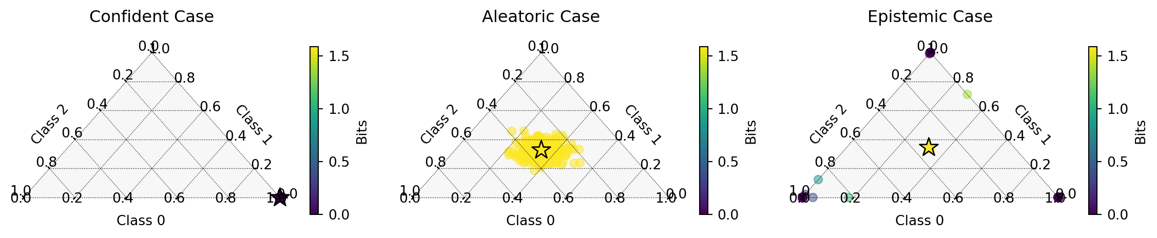
| Case | Predicted Class | Confidence | Total Uncertainty | Aleatoric Uncertainty | Epistemic Uncertainty |
|---|---|---|---|---|---|
| Confident | 0 | 1.000 | 0.000 | 0.000 | 0.000 |
| Aleatoric | 0 | 0.336 | 1.099 | 1.083 | 0.016 |
| Epistemic | 1 | 0.346 | 1.098 | 0.014 | 1.084 |
Laplace Approximation
The Core Idea
- Approximate the posterior \(\pof{\w \given \D}\) with a Gaussian distribution
- Uses a second-order Taylor expansion around information content of MAP estimate \(\wstar\)
- Results in \(\qof{\w} = \mathcal{N}(\wstar, \HofHessian{\wstar}^{-1})\)
What is \(\HofHessian{\wstar}\) though?
Notation
We write \(\HofJacobian{\cdot}\) and \(\HofHessian{\cdot}\) for the Jacobian and Hessian of the negative log probability of \(\cdot\).
\[ \begin{aligned} \HofJacobian{\cdot} &\coloneqq \nabla_{\w} [\Hof{\cdot}] \\ \HofHessian{\cdot} &\coloneqq \nabla^2_{\w} [\Hof{\cdot}]. \end{aligned} \]
Notation
We write \(\HofJacobian{\cdot}\) and \(\HofHessian{\cdot}\) for the Jacobian and Hessian of the negative log probability of \(\cdot\).
\[ \begin{aligned} \HofJacobian{\cdot} &\coloneqq \nabla_{\w} [\Hof{\cdot}] = -\nabla_{\w} \log \pof{\cdot} \\ \HofHessian{\cdot} &\coloneqq \nabla^2_{\w} [\Hof{\cdot}] = -\nabla^2_{\w} \log \pof{\cdot}. \end{aligned} \]
Second-Order Taylor Expansion - Take 1
Around the information content of \(\wstar\):
\[ \begin{aligned} &- \log \pof{\w \given \D} \\ &\quad \approx - \log \pof{\wstar \given \D} \\ &\quad \phantom{\approx} + (\w - \wstar)^T \nabla_{\w} [-\log \pof{\wstar \given \D}] \\ &\quad \phantom{\approx}+ \frac{1}{2}(\w - \wstar)^T \nabla^2_{\w} [-\log \pof{\wstar \given \D}] (\w - \wstar) \\ &\quad \phantom{\approx}+ \mathcal{O}(\|\w - \wstar\|^3). \end{aligned} \]
Completing the Square
For a quadratic form, we can complete the square:
\[ \begin{aligned} \frac{1}{2} x^T A x + b^T x + c &= \frac{1}{2}(x + A^{-1}b)^T A (x + A^{-1}b) \\ &\phantom{=} - \frac{1}{2}b^T A^{-1}b + c \\ &= \frac{1}{2}(x - \mu)^T A (x - \mu) + \text{const}, \end{aligned} \]
with \(\mu \coloneqq -A^{-1}b\).
Completing the Square - Take 1
\[ \begin{aligned} &\phantom{=} -\log \pof{\wstar} + \nabla_{\w}[-\log \pof{\wstar}](\w - \wstar) + \frac{1}{2}(\w - \wstar)^T \nabla^2_{\w}[-\log \pof{\wstar}] (\w - \wstar) \\ &= -\log \pof{\wstar} + \frac{1}{2}\left[2\nabla_{\w}[-\log \pof{\wstar}](\w - \wstar) + (\w - \wstar)^T \nabla^2_{\w}[-\log \pof{\wstar}] (\w - \wstar)\right] \\ &= -\log \pof{\wstar} + \frac{1}{2}\left[(\w - \mu)^T \nabla^2_{\w}[-\log \pof{\wstar}] (\w - \mu)\right] + \text{const} \end{aligned} \]
where \(\mu \coloneqq \wstar - \nabla^2_{\w}[-\log \pof{\wstar}]^{-1}\nabla_{\w}[-\log \pof{\wstar}]\) will be the mean of the Gaussian.
Second-Order Taylor Expansion
Now using the notation with \(\HofJacobian{\cdot}\) and \(\HofHessian{\cdot}\):
\[ \begin{aligned} \Hof{\w} &= \Hof{\wstar} + \HofJacobian{\wstar}(\w - \wstar) \\ &\quad + \frac{1}{2}(\w - \wstar)^T \HofHessian{\wstar} (\w - \wstar) \\ &\quad + \mathcal{O}(\|\w - \wstar\|^3). \end{aligned} \]
Completing the Square - Take 2
For a quadratic form with our notation:
\[ \begin{aligned} \Hof{\w} &= \Hof{\wstar} + \HofJacobian{\wstar}(\w - \wstar) \\ &\quad + \frac{1}{2}(\w - \wstar)^T \HofHessian{\wstar} (\w - \wstar) \\ &\quad + \mathcal{O}(\|\w - \wstar\|^3). \end{aligned} \]
Tip
\[ \begin{aligned} \frac{1}{2} x^T A x + b^T x + c &= \frac{1}{2}(x + A^{-1}b)^T A (x + A^{-1}b) \\ &\phantom{=} - \frac{1}{2}b^T A^{-1}b + c \\ &= \frac{1}{2}(x - \mu)^T A (x - \mu) + \text{const}, \end{aligned} \]
with \(\mu \coloneqq -A^{-1}b\).
\[ \begin{aligned} \Hof{\w} &= \frac{1}{2}(\w - \mu)^T \HofHessian{\wstar} (\w - \mu) \\ &\quad + \text{const} + \mathcal{O}(\|\w - \wstar\|^3), \end{aligned} \]
where \(\mu \coloneqq \wstar - \HofHessian{\wstar}^{-1}\HofJacobian{\wstar}\).
\(\rightsquigarrow\) Probability Distribution
Turning this into a probability distribution:
\[ \begin{aligned} &\pof{\w} = \exp(-\Hof{\w}) \\ &\quad \approx \exp\left(-\frac{1}{2}(\w - \mu)^T \HofHessian{\wstar} (\w - \mu) + \text{ const} \right), \end{aligned} \]
with \(\mu \coloneqq \wstar - \HofHessian{\wstar}^{-1}\HofJacobian{\wstar}\).
This matches the form of a Gaussian with mean \(\wstar\) and covariance \(\HofHessian{\wstar \given \D}^{-1}\) up to a constant:
Laplace Approximation
This matches the form of a Gaussian with mean \(\wstar\) and covariance \(\HofHessian{\wstar \given \D}^{-1}\) up to a constant:
\[ \begin{aligned} \qof{\w} &= \mathcal{N}(\wstar - \HofHessian{\wstar}^{-1}\HofJacobian{\wstar}, \HofHessian{\wstar}^{-1}) \\ &\propto \exp\left(-\frac{1}{2}(\w - \mu)^T \HofHessian{\wstar} (\w - \mu) + \text{ const} \right) \\ &\approx \pof{\w}. \end{aligned} \]
Summary
The Laplace approximation is the Gaussian distribution that best approximates the information content of \(\pof{\w}\) using the second-order Taylor expansion.
\[ \qof{\w} = \mathcal{N}(\wstar - \HofHessian{\wstar}^{-1}\HofJacobian{\wstar}, \HofHessian{\wstar}^{-1}). \]
The Posterior Approximation
The Laplace approximation for the posterior at \(\wstar\)gives us:
\[ \pof{\w \given \D} \approx \mathcal{N}(\wstar - \HofHessian{\wstar \given \D}^{-1}\HofJacobian{\wstar \given \D}, \HofHessian{\wstar \given \D}^{-1}) \]
where:
- \(\wstar\) is the MAP estimate (mode of posterior)
- \(\HofHessian{\wstar}\) is the Hessian of the information content of \(\pof{\cdot \given \D}\) at \(\wstar\)
The MAP Estimate
The MAP estimate is the \(\wstar\) that minimizes the objective \(\Hof{\w \given \D}\).
Hence, \(\HofJacobian{\wstar} = 0.\), and we have
\[ \Hof{\w \given \D} \approx \frac{1}{2}(\w - \wstar)^T \HofHessian{\wstar \given \D} (\w - \wstar) + \text{ const }. \]
Therefore, the Laplace approximation for the posterior at \(\wstar\) simplifies to: \[ \pof{\w \given \D} \approx \mathcal{N}(\wstar, \HofHessian{\wstar \given \D}^{-1}). \]
Decomposing the Hessian
Using Bayes’ rule:
\[ \begin{aligned} \HofHessian{\wstar \given \D} &= \HofHessian{\D \given \wstar} + \HofHessian{\wstar} \\ &= \text{likelihood Hessian} + \text{prior Hessian} \end{aligned} \]
One More Time
\[ \begin{aligned} \HofHessian{\wstar \given \D} &= \HofHessian{\frac{\pof{\D \given \wstar} \pof{\wstar}}{\pof{\D}}} \\ &= \HofHessian{\pof{\D \given \wstar}} + \HofHessian{\pof{\wstar}} - \HofHessian{\pof{\D}} \\ &= \HofHessian{\D \given \wstar} + \HofHessian{\wstar} + 0 \end{aligned} \]
Why?
\(\HofHessian{\D}\) is independent of \(\w\), so the Jacobian and Hessian vanish.
Liklihood Hessian
The likelihood Hessian is the Hessian of the negative log likelihood of the data given the parameters:
\[ \begin{aligned} \HofHessian{\D \given \w} &= \nabla^2_{\w} \left[ - \log \pof{\D \given \w} \right] \\ &= \sum_{i=1}^n \nabla^2_{\w} \left[ - \log \pof{\y_i \given \x_i, \w} \right]. \end{aligned} \]
Summary
Now, we have all the ingredients to compute the Laplace approximation for the posterior.
We compute the prior Hessian \(\HofHessian{\wstar}\) and the likelihood Hessian \(\HofHessian{\D \given \wstar}\) and together they give us the Laplace approximation for the posterior.
Practical Implementation
def apply_laplace_approximation(model, train_loader):
    """Apply Laplace approximation using GGN"""
    la = Laplace(
        model,
        likelihood='classification',
        subset_of_weights='all',
        hessian_structure='gp',
        backend=CurvlinopsGGN
    )
    # Fit and optimize
    la.fit(train_loader)
    la.optimize_prior_precision()
    return la
Generalized Gauss-Newton Approximation
For better numerical stability, we often approximate:
\[ \begin{aligned} \HofHessian{\y \given \x, \wstar} &\approx \HofHessian{\Y \given \x, \wstar} \\ &\coloneqq \E{\pof{\y \given \x, \wstar}}{\HofHessian{\y \given \x, \wstar}}. \end{aligned} \]
This ensures positive definiteness of the Hessian approximation.
What? Why?
\(\HofHessian{\Y \given \x, \wstar}\) is often easier to compute than \(\HofHessian{\w \given \D}\).
There exist simple closed-form solutions for many common likelihoods.
Gaussian Regression
For Gaussian regression with variance \(\sigma^2\):
\[ \y \sim \mathcal{N}(f(\x, \wstar), \sigma^2), \]
the Fisher Information is:
\[ \begin{aligned} \HofHessian{\Y \given \x, \wstar} = \frac{1}{\sigma^2} \nabla f(\x, \wstar) \nabla f(\x, \wstar)^\top, \end{aligned} \]
where \(f(\x, \wstar)\) is the network output at the MAP estimate.
Multi-class Classification
For multi-class classification with softmax likelihood:
\[ \y \sim \text{Cat}(\text{softmax}(f(\x, \wstar))), \]
we have:
\[ \newcommand{\J}{\mathbf{J}} \newcommand{\p}{\mathbf{p}} \begin{aligned} \HofHessian{\Y \given \x, \wstar} &= \J^\top \text{diag}(\p) \J - \J^\top(\p\p^\top)\J, \end{aligned} \]
where:
- \(\J = \nabla f(\x, \wstar)\) is the Jacobian of logits with respect to parameters
- \(\p = \text{softmax}(f(\x, \wstar))\) is the vector of predicted probabilities
- \(\text{diag}(\p)\) is a diagonal matrix with entries from \(\p\)
Limitations & Considerations
- Assumes posterior is approximately Gaussian
- Quality depends on:
- Amount of data
- Model architecture
- Parameter dimensionality
- May underestimate uncertainty in multimodal posteriors
- Computationally efficient compared to full VI
Best Practices
- Use GGN approximation for stability
- Verify positive definiteness of Hessian
- Be cautious with limited data
Fisher Information
The quantity \(\HofHessian{\Y \given \x, \wstar}\) is also known as the Fisher Information.
Definition 2 The Fisher Information is the expected Hessian of the negative log likelihood of the data given the parameters:
\[ \HofHessian{\Y \given \x, \wstar} \coloneqq \E{\pof{\y \given \x, \wstar}}{\HofHessian{\y \given \x, \wstar}}. \]
Observed Information
The quantity \(\HofHessian{\y \given \x, \wstar}\) is also known as the observed Information.
Definition 3 The Observed Information is the Hessian of the negative log likelihood of the data given the parameters:
\[ \HofHessian{\y \given \x, \wstar} \coloneqq \nabla^2_{\w} \left[ - \log \pof{\y \given \x, \w} \right]. \]
Conclusion
What You Can Now Do
- Understand Different Uncertainty Types
- Distinguish between aleatoric and epistemic uncertainty
- Recognize when each type matters for your application
- Choose Appropriate Methods
- Select between density-based, variational, and Laplace approaches
- Understand tradeoffs in computational cost vs accuracy
- Implement Uncertainty Quantification
- Use Monte Carlo Dropout for quick uncertainty estimates
- Apply DDU for efficient density-based uncertainty
- Implement Laplace approximation for post-hoc uncertainty
- Apply to Real Problems
- Detect out-of-distribution samples
- Guide active learning acquisition
- Provide reliable confidence estimates
Key Takeaways
- No method is perfect
- Simple methods (MC Dropout, DDU) often work well in practice
- Understanding the theory helps make better implementation choices
- Always validate uncertainty estimates empirically
Remember
Uncertainty quantification is crucial for deploying ML systems responsibly!
Appendix
Good Overview Paper
The paper 🪧 by Hüllermeier and Waegeman (2021) gives a great overview of the different types of uncertainty and how to estimate them. Beyond Bayesian methods, it also covers conformal prediction and credal sets as alternative approaches in an introductory manner.
As podcast (created using NotebookLM):
References
Blundell, Charles, Julien Cornebise, Koray Kavukcuoglu, and Daan Wierstra. 2015. “Weight Uncertainty in Neural Network.” In International Conference on Machine Learning, 1613–22. PMLR.
Box, George EP, and WILLIAM J Hill. 1967. “Discrimination Among Mechanistic Models.” Technometrics 9 (1): 57–71.
Gal, Yarin, and Zoubin Ghahramani. 2016. “Dropout as a Bayesian Approximation: Representing Model Uncertainty in Deep Learning.” In International Conference on Machine Learning, 1050–59. PMLR.
Hüllermeier, Eyke, and Willem Waegeman. 2021. “Aleatoric and Epistemic Uncertainty in Machine Learning: An Introduction to Concepts and Methods.” Machine Learning 110 (3): 457–506.
Immer, Alexander, Maciej Korzepa, and Matthias Bauer. 2021. “Improving Predictions of Bayesian Neural Nets via Local Linearization.” In International Conference on Artificial Intelligence and Statistics, 703–11. PMLR.
Kendall, Alex, and Yarin Gal. 2017. “What Uncertainties Do We Need in Bayesian Deep Learning for Computer Vision?” Advances in Neural Information Processing Systems 30.
Kingma, Diederik P. 2013. “Auto-Encoding Variational Bayes.” arXiv Preprint arXiv:1312.6114.
Kirsch, Andreas. 2024. “Advancing Deep Active Learning & Data Subset Selection: Unifying Principles with Information-Theory Intuitions.” arXiv Preprint arXiv:2401.04305.
Lakshminarayanan, Balaji, Alexander Pritzel, and Charles Blundell. 2016. “Simple and Scalable Predictive Uncertainty Estimation Using Deep Ensembles. arXiv e-Prints, Art.” arXiv Preprint arXiv:1612.01474.
Lindley, Dennis V. 1956. “On a Measure of the Information Provided by an Experiment.” The Annals of Mathematical Statistics 27 (4): 986–1005.
MacKay, David JC. 1992. “Information-Based Objective Functions for Active Data Selection.” Neural Computation 4 (4): 590–604.
Song, Junho, Woojin Ahn, Sangkyoo Park, and Myotaeg Lim. 2021. “Failure Detection for Semantic Segmentation on Road Scenes Using Deep Learning.” Applied Sciences 11 (4): 1870.