Information Theory
Introduction
Andreas Kirsch
Why Information Theory?
Real-World Impact
Information theory powers modern compression algorithms like ZIP files, image compression (JPEG), and is fundamental to machine learning. Active learning is a prime example of how information theory can be applied to improve learning systems.
What You’ll Learn Today
\[ \require{mathtools} \DeclareMathOperator{\opExpectation}{\mathbb{E}} \newcommand{\E}[2]{\opExpectation_{#1} \left [ #2 \right ]} \newcommand{\simpleE}[1]{\opExpectation_{#1}} \newcommand{\implicitE}[1]{\opExpectation \left [ #1 \right ]} \DeclareMathOperator{\opVar}{\mathrm{Var}} \newcommand{\Var}[2]{\opVar_{#1} \left [ #2 \right ]} \newcommand{\implicitVar}[1]{\opVar \left [ #1 \right ]} \newcommand\MidSymbol[1][]{% \:#1\:} \newcommand{\given}{\MidSymbol[\vert]} \DeclareMathOperator{\opmus}{\mu^*} \newcommand{\IMof}[1]{\opmus[#1]} \DeclareMathOperator{\opInformationContent}{H} \newcommand{\ICof}[1]{\opInformationContent[#1]} \newcommand{\xICof}[1]{\opInformationContent(#1)} \newcommand{\sicof}[1]{h(#1)} \DeclareMathOperator{\opEntropy}{H} \newcommand{\Hof}[1]{\opEntropy[#1]} \newcommand{\xHof}[1]{\opEntropy(#1)} \DeclareMathOperator{\opMI}{I} \newcommand{\MIof}[1]{\opMI[#1]} \DeclareMathOperator{\opTC}{TC} \newcommand{\TCof}[1]{\opTC[#1]} \newcommand{\CrossEntropy}[2]{\opEntropy(#1 \MidSymbol[\Vert] #2)} \DeclareMathOperator{\opKale}{D_\mathrm{KL}} \newcommand{\Kale}[2]{\opKale(#1 \MidSymbol[\Vert] #2)} \DeclareMathOperator{\opJSD}{D_\mathrm{JSD}} \newcommand{\JSD}[2]{\opJSD(#1 \MidSymbol[\Vert] #2)} \DeclareMathOperator{\opp}{p} \newcommand{\pof}[1]{\opp(#1)} \newcommand{\pcof}[2]{\opp_{#1}(#2)} \newcommand{\hpcof}[2]{\hat\opp_{#1}(#2)} \DeclareMathOperator{\opq}{q} \newcommand{\qof}[1]{\opq(#1)} \newcommand{\qcof}[2]{\opq_{#1}(#2)} \newcommand{\varHof}[2]{\opEntropy_{#1}[#2]} \newcommand{\xvarHof}[2]{\opEntropy_{#1}(#2)} \newcommand{\varMIof}[2]{\opMI_{#1}[#2]} \DeclareMathOperator{\opf}{f} \newcommand{\fof}[1]{\opf(#1)} \newcommand{\indep}{\perp\!\!\!\!\perp} \newcommand{\Y}{Y} \newcommand{\y}{y} \newcommand{\X}{\boldsymbol{X}} \newcommand{\x}{\boldsymbol{x}} \newcommand{\w}{\boldsymbol{\theta}} \newcommand{\W}{\boldsymbol{\Theta}} \newcommand{\wstar}{\boldsymbol{\theta^*}} \newcommand{\D}{\mathcal{D}} \newcommand{\HofHessian}[1]{\opEntropy''[#1]} \newcommand{\specialHofHessian}[2]{\opEntropy''_{#1}[#2]} \newcommand{\HofJacobian}[1]{\opEntropy'[#1]} \newcommand{\specialHofJacobian}[2]{\opEntropy'_{#1}[#2]} \newcommand{\indicator}[1]{\mathbb{1}\left[#1\right]} \]
After this lecture, you’ll be able to:
- Design optimal codes for data compression
- Calculate the theoretical limits of compression
- Understand why certain codes are better than others
- Apply information theory concepts to real-world problems
Lecture Roadmap
- Motivation
- Real-world compression examples
- Why we need information theory
- Core Concepts
- Information content
- Entropy basics
- Simple coding examples
- Coding Techniques
- Fixed vs variable length
- Huffman coding
- Practical examples
- Theory & Proofs
- Kraft’s inequality
- Source coding theorems
- Information Quantities
- Joint Entropy
- Mutual information
- Conditional entropy
- Chain rule
- Information Diagrams
- Practice
- Theory
Introduction
Information theory helps us:
- Quantify information content of random variables and events
- Provide valuable insights and intuitions
- Offer a principled framework for reasoning about uncertainty
Information theory is widely used in machine learning for/with:
- Learning via compression
- Information bottlenecks in supervised/unsupervised learning
- Bayesian experimental design
- Active learning
- Submodularity
Common Misconceptions
Warning
Information theory is NOT:
- Just about compression
- Limited to computer science
- Only about binary codes
- The same as classical probability theory
Common Challenges
Common challenges when learning information theory:
- Ambiguity in complex expressions
- Deviation between fields (statistics, CS, information engineering)
- Confusion between cross-entropy and joint entropy
- Unclear expectations over random variables
Example of Ambiguity
\(H(X,Y)\) could mean:
- Joint entropy of X and Y
- Cross-entropy between X and Y
Probability & Information Theory
- Information theory builds on probability theory to quantify uncertainty and information
- Probability distributions determine how much information we gain from observing outcomes
- Less probable events carry more information (seeing a rare event tells us more than a common one)
- The entropy of a distribution measures its inherent uncertainty
- Mutual information quantifies how much uncertainty in one variable is reduced by knowing another
Key Connection
Information theory provides a mathematical framework for measuring the “surprise value” of probabilistic events. The more unlikely an event, the more informative it is when it occurs.
Review: Probability
Information theory builds on probability theory to quantify uncertainty and information.
Important
Understanding these basics is crucial for information theory!
Probability Distributions
Let’s review some basic probability distributions and concepts.
- For discrete random variable \(X\): \(\pof{X=x}\) is the probability of outcome \(x\).
- For continuous variables, \(\pof{X=x}\) is the probability density function, and e.g. \(\pof{X \in [a,b]}\) is the probability mass of the interval \([a,b]\).
Notation
We write \(\pof{x}\) as shorthand for \(\pof{X=x}\).
Key Concepts
For any random variables \(A\) and \(B\):
Conditional Probability
\[ \pof{b \given a} = \frac{\pof{a,b}}{\pof{a}} \]
Independence
\[ \pof{a,b} = \pof{a} \pof{b} \quad \forall a,b \]
We write: \(A \indep B\) if \(\pof{a,b} = \pof{a} \pof{b}\).
Law of Total Probability
\[ \pof{b} = \sum_a \pof{b \given a} \,\pof{a}. \]
Bayes’ Theorem
\[ \pof{A \given B} = \frac{\pof{B \given A}\pof{A}}{\pof{B}} \]
Example: Email Spam Filter
For a spam email (S) containing word “money” (M):
| Term | Notation | Meaning |
|---|---|---|
| \(\pof{S}\) | 0.3 | 30% of all emails are spam |
| \(\pof{M \given S}\) | 0.6 | 60% of spam emails contain “money” |
| \(\pof{M \given \neg S}\) | 0.05 | 5% of non-spam emails contain “money” |
| \(\pof{S \given M}\) | ??? | What fraction of emails with “money” are spam? |
We can find \(\pof{M}\) using the law of total probability:
\[ \begin{aligned} \pof{M} &= \pof{M \given S}\pof{S} + \pof{M \given \neg S}\pof{\neg S} \\ &= 0.6 \cdot 0.3 + 0.05 \cdot 0.7 \\ &= 0.215 \end{aligned} \]
Now we can apply Bayes’ theorem: \[ \pof{S \given M} = \frac{\pof{M \given S}\,\pof{S}}{\pof{M}} = \frac{0.6 \cdot 0.3}{0.215} \approx 0.84 \]
Bayesian Inference
Bayes’ theorem also shows how to update probabilities when new evidence arrives. It connects:
\[ \pof{A \given B} = \frac{\pof{B \given A}\pof{A}}{\pof{B}} \]
- Prior belief: \(\pof{A}\)
- Likelihood of evidence: \(\pof{B \given A}\)
- Posterior belief: \(\pof{A \given B}\)
Example: Medical Testing
For a disease (D) and positive test (T):
| Term | Notation | Meaning |
|---|---|---|
| Prior | \(\pof{D}\) | Disease prevalence |
| Likelihood | \(\pof{T \given D}\) | Test sensitivity |
| Posterior | \(\pof{D \given T}\) | Diagnosis confidence |
Expected Value & Variance
\[ \begin{aligned} \implicitE{X} &= \sum_{x} x\pof{x} \text{ or } \int x\pof{x}dx \\ \implicitVar{X} &= \implicitE{(X-\implicitE{X})^2} = \implicitE{X^2} - \implicitE{X}^2 \end{aligned} \]
Notation for Expectations
- \(\implicitE{X}\) denotes the expectation of a random variable \(X\) over the “corresponding” distribution \(\pof{x}\) (implicitly).
- \(\E{\pof{x}}{x}\) denotes the expectation of a random variable \(X\) over the distribution \(\pof{x}\) explicitly. We use a lower-case \(x\) to indicate that the \(x\) is bound to \(x \sim \pof{x}\). It is essentially a short-hand for \(\int\) or \(\sum\).
- Same for \(\implicitVar{X}\) (and \(\Var{\pof{x}}{x}\)—but I don’t think we’ll see that).
Discrete Probability Distributions
Models single trial success/failure of probability \(p\)
| Property | Formula |
|---|---|
| Probability mass function | \(\pof{X=1} = p\), \(\pof{X=0} = 1-p\) |
| Mean | \(\implicitE{X} = p\) |
| Variance | \(\implicitVar{X} = p(1-p)\) |
from scipy.stats import bernoulli
# Probability mass function
bernoulli_probs = bernoulli.pmf([0, 1], p)
# Drawing samples
bernoulli_samples = bernoulli.rvs(p, size)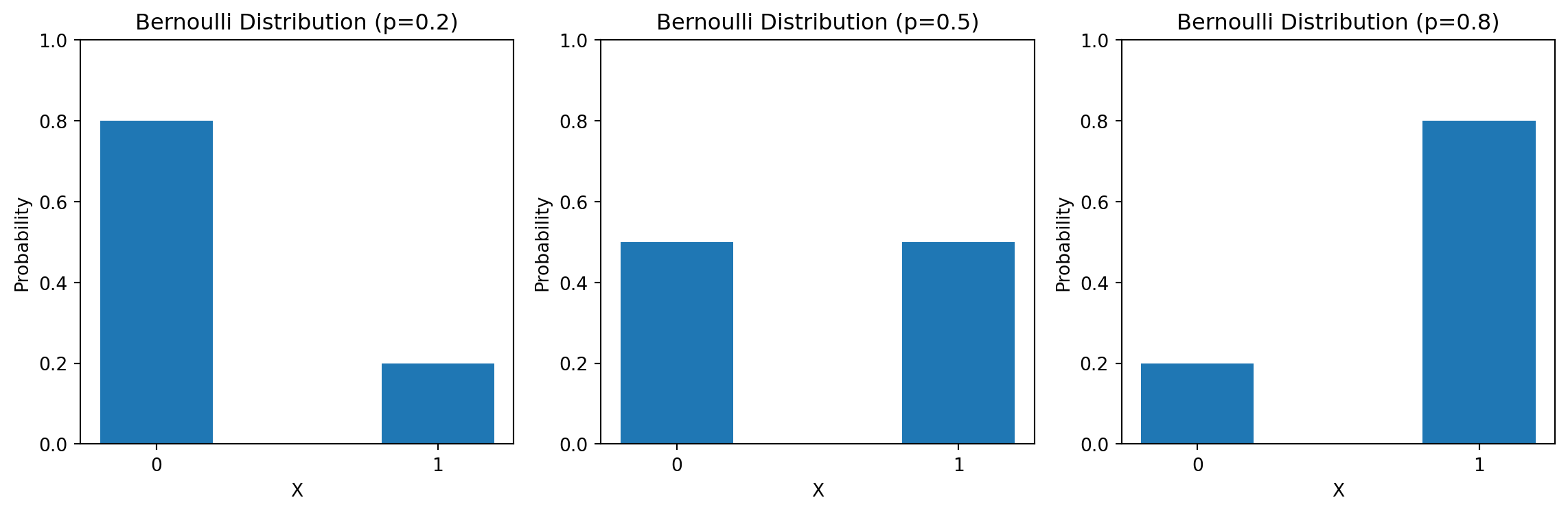
Counts successes in \(n\) independent Bernoulli trials of probability \(p\)
| Property | Formula |
|---|---|
| Probability mass function | \(\pof{X=k} = \binom{n}{k} \, p^k(1-p)^{n-k}\) |
| Mean | \(\implicitE{X} = np\) |
| Variance | \(\implicitVar{X} = np(1-p)\) |
from scipy.stats import binom

# Probability mass function
binomial_probs = binom.pmf(np.arange(0, n+1), n, p)
# Drawing samples
binomial_samples = binom.rvs(n, p, size)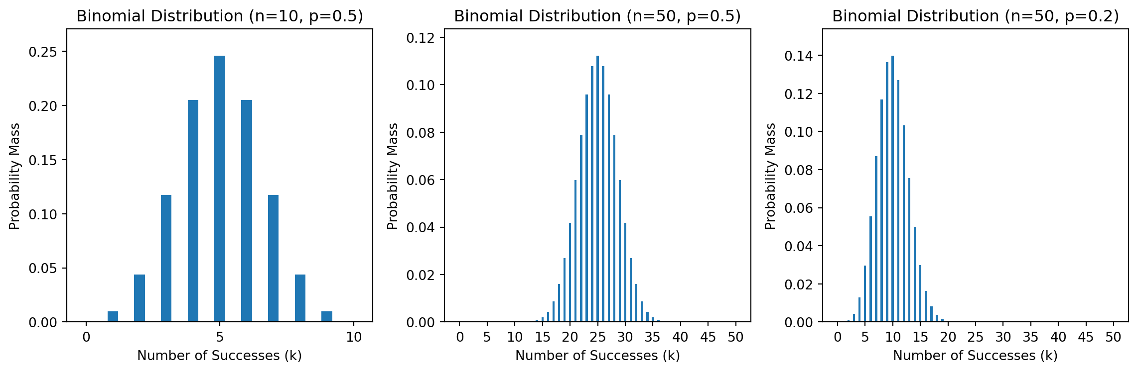
Continuous Probability Distributions
Models uniform probability over interval \([a,b]\)
| Property | Formula |
|---|---|
| Probability density function | \(\pof{X=x} = \frac{1}{b-a}\) for \(x \in [a,b]\) |
| Mean | \(\implicitE{X} = \frac{a+b}{2}\) |
| Variance | \(\implicitVar{X} = \frac{(b-a)^2}{12}\) |
from scipy.stats import uniform

# PDF evaluation
x = np.linspace(a-1, b+1, 100)
uniform_pdf = uniform.pdf(x, loc=a, scale=b-a)
# Generate samples
uniform_samples = uniform.rvs(loc=a, scale=b-a, size=1000)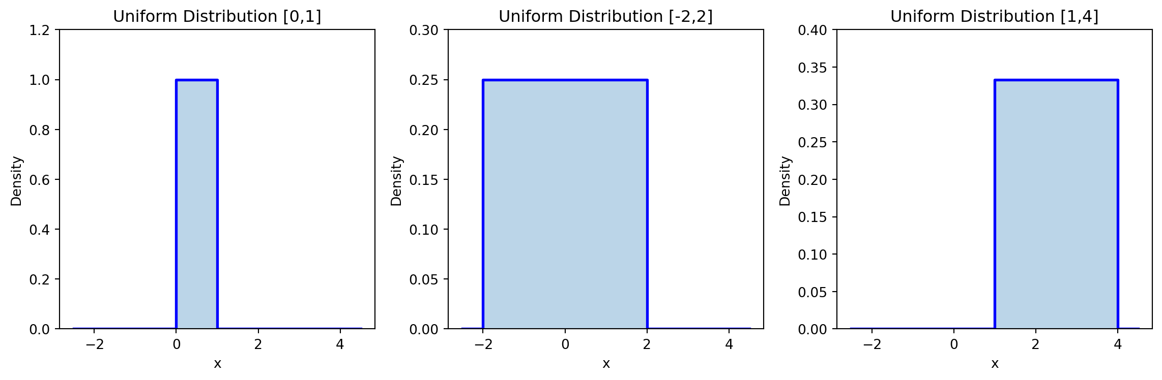
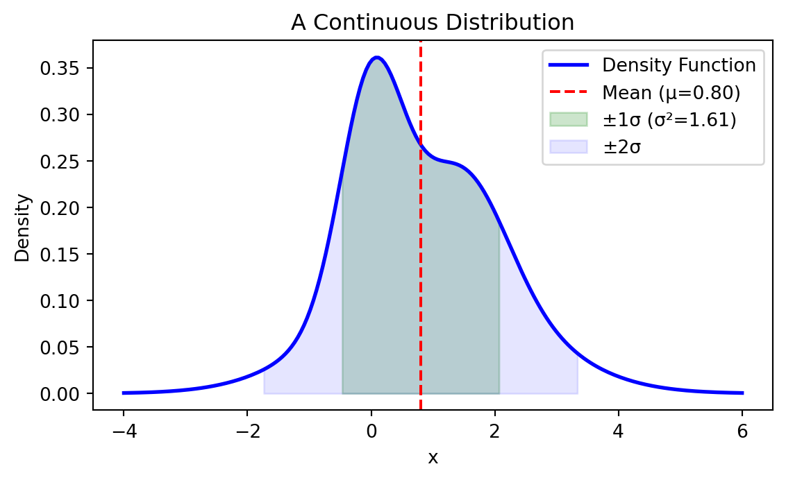
Bell-shaped curve characterized by mean \(\mu\) and variance \(\sigma^2\)
| Property | Formula |
|---|---|
| Probability density function | \(\pof{X=x} = \frac{1}{\sqrt{2\pi\sigma^2}}e^{-\frac{(x-\mu)^2}{2\sigma^2}}\) |
| Mean | \(\implicitE{X} = \mu\) |
| Variance | \(\implicitVar{X} = \sigma^2\) |
from scipy.stats import norm

# Generate samples
gaussian_samples = norm.rvs(loc=mu, scale=sigma, size=1000)
# PDF evaluation
x = np.linspace(mu-4*sigma, mu+4*sigma, 100)
gaussian_pdf = norm.pdf(x, loc=mu, scale=sigma)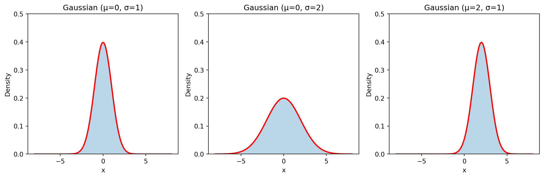
Interactive Demo
Information Content
Information Content
How do we measure the information content of an event?
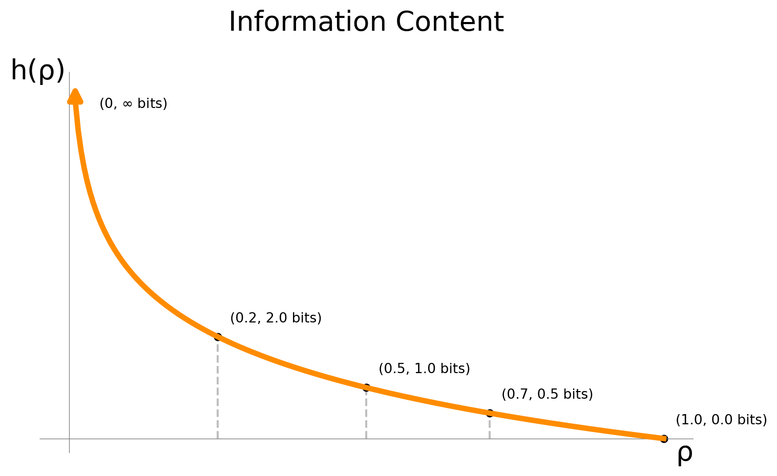
Shannon’s information content for an event \(x\):
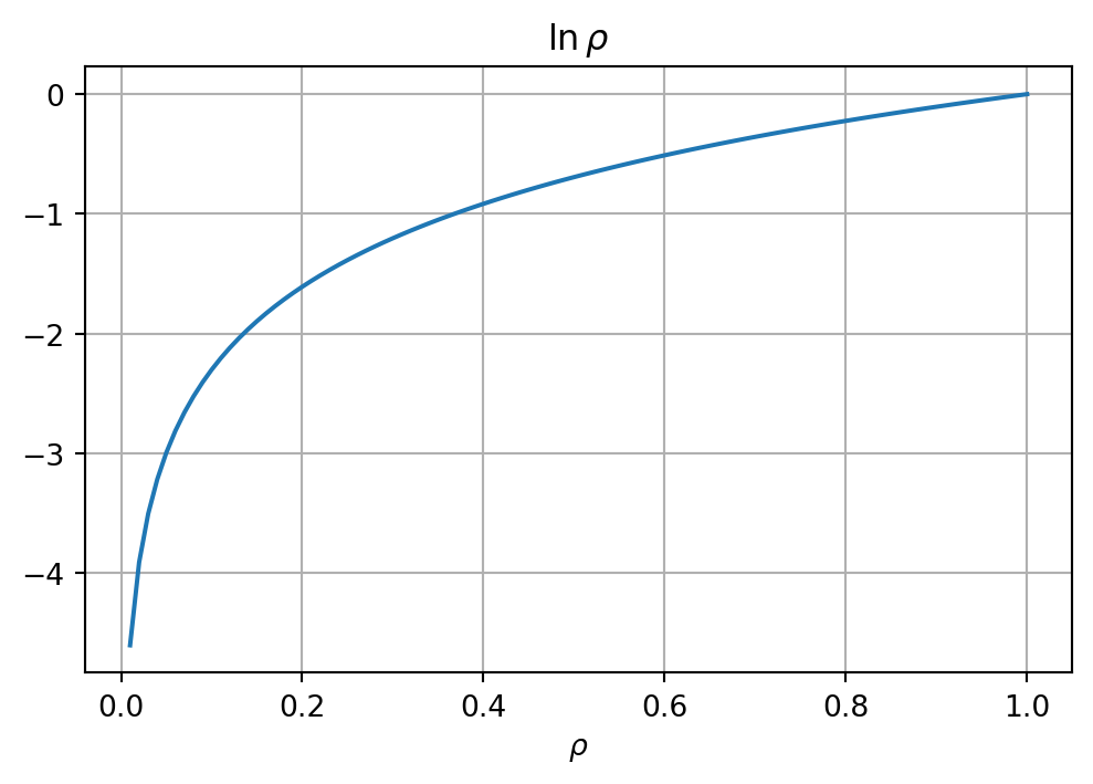
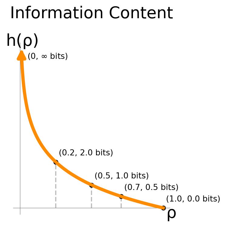
\[ \xHof{\pof{x}} = -\ln(\pof{x}). \]
(Or simpler: \(\sicof{\rho} = -\ln(\rho).\))
Wait, but why?
Desirable Properties of \(\sicof{\pof{x}}\)
The information content of an event is always relative to a set of events (e.g. outcomes of a discrete R.V.). We want the information content to be:
a continuous function of the probability of the event,
montonously decreasing—the less probable an event, the more information it carries: \[\pof{x_1} < \pof{x_2} \implies \sicof{\pof{x_1}} > \sicof{\pof{x_2}},\]
additive for independent events: \[ x \indep y \implies \sicof{\pof{x,y}} = \sicof{\pof{x}} + \sicof{\pof{y}}. \]
Let’s solve this (assuming diff’able)
If \(x \indep y\), then \(\pof{x,y} = \pof{x}\pof{y}\), so we need to have:
\[ \sicof{\pof{x} \pof{y}} = \sicof{\pof{x}} + \sicof{\pof{y}}. \]
W.l.o.g., let \(a := \pof{x}\) and \(b := \pof{y}\). Then we need:
\[ \begin{aligned} \sicof{a \, b} &= \sicof{a} + \sicof{b} \\ \implies \frac{d}{db} \sicof{a \, b} &= \frac{d}{db} \sicof{a} + \frac{d}{db} \sicof{b} \end{aligned} \]
\[ \implies a h'(a b) = h'(b) \implies h'(a b) = \frac{h'(b)}{a}. \]
Let’s fix \(b:=1\) and define \(h'(1) := c\). Then we have:
\[ h'(a) = \frac{c}{a}. \]
\[ \implies h(a) - h(1) = \int_1^a \frac{c}{x} dx = c \ln a. \]
So we have:
\[ h(a) = c \ln a + h(1). \]
What is \(h(1)\)?
\[ h(a \, b) = h(a) + h(b) = c \ln a + c \ln b + 2\, h(1), \]
but also:
\[ h(a \, b) = c \ln (a b) + h(1) = c \ln a + c \ln b + h(1). \]
\[ \implies h(1) = 0. \]
Thus, we have:
\[ h(a) = c \ln a. \]
How do we choose \(c\)?
To be monotonically decreasing, we need \(c<0\) because \(\ln(a)\) is monotonically increasing.
Final Functional Form
We can choose \(c:=-1\) to get the simplest expression:
Important
\[ \sicof{\rho} = -\ln \rho. \]
Nats vs Bits
The information content is dimensionless, but we will use a pseudo-unit for it called nats.
If we picked \(\sicof{\rho} = -\log_2 \rho\), we would use bits as unit.
The difference is a factor of \(\ln 2\): \[ 1 \text{ bit} = \ln 2 \text{ nat} \approx 0.6931 \text{ nat}. \]
Why Bits?
Given a uniform distribution, what’s the information content of a specific 4-bit string?
4-bit strings: \(2^4 = 16\) possible outcomes.
\[ \implies \pof{x} = \frac{1}{2^4} = \frac{1}{16}. \]
\[ \implies \sicof{\pof{x}} = -\ln \left( \frac{1}{2^4} \right) \]
\[ = 4 \ln 2 \text{ nats} = 4 \text{ bits}. \]
Why Bits?
Given a uniform distribution, what’s the information content of a specific 4-bit string?
Important
A 4-bit string contains exactly 4 bits of information!
Why Bits?
Note
A fair coin-flip contains \(\boxed{?}\) bit of information.
Why Bits?
Note
A fair coin-flip contains \(\boxed{1}\) bit of information.
Shannon’s Information Content
For an event with probability \(\rho\), the information content is:
\[\sicof{\rho} = -\ln \rho.\]
Key properties:
Decreases monotonically with probability
Approaches infinity as \(\rho \to 0\)
Equals zero when \(\rho = 1\)
Additive for independent events:
\[ \sicof{\rho_1 \rho_2} = \sicof{\rho_1} + \sicof{\rho_2} \]
(Towards) Compression
We have seen that for a uniform distribution, the information content can be related to the number of bits needed to encode a specific outcome.
Is this the best we can do? And what if the distribution is not uniform?
Information Content as a Lower Bound
Important
On average, the information content of a specific outcome is a lower bound on the number of bits needed to encode it.
Note
We could cheat and try to encode one outcome with fewer bits, but then we’d pay for it with other outcomes, and on average we’d be worse off.
Codes
A code maps source symbols to sequences of symbols from a code alphabet. The goal is typically to:
- Represent information efficiently (minimize average sequence length)
- Enable reliable transmission (protect against errors)
Key Terminology
Symbol: A basic unit of information (e.g., a letter, digit, or voltage level)
Alphabet: A finite set of symbols
- Example 1: Binary alphabet {0,1}
- Example 2: English alphabet {A,B,…,Z}
String: A finite sequence of symbols from an alphabet
- Example 1: “101001” (binary string)
- Example 2: “HELLO” (text string)
Code: A system that converts symbols from one alphabet into strings of symbols from another alphabet
Example 1: ASCII Code
- Source symbols: Text characters
- Code alphabet: Binary digits (0 and 1)
- Mapping: Each character is converted to an 8-digit binary string
- Example: ‘A’ is converted to ‘01000001’
Example 2: Morse Code
- Source symbols: Letters and numbers
- Code alphabet: {dot (.), dash (-), space}
- Mapping: Each character is converted to a sequence of dots and dashes
- Examples:
- ‘E’ → ‘.’ (most common English letter: shortest code)
- ‘A’ → ‘.-’
- ‘B’ → ‘-…’
- ‘SOS’ → ‘… — …’ (famous distress signal)
- (What is ’ ’ →?)
Formal Definitions
Let’s formalize these concepts:
Alphabet: A finite set of symbols, denoted \(\mathcal{A}\)
Strings: A finite sequence of symbols from \(\mathcal{A}\)
- Set of all finite strings over \(\mathcal{A}\) denoted by \(\mathcal{A}^*\)
- Length of string \(x\) denoted by \(|x|\)
- Empty string denoted by \(\epsilon\)
- Example: If \(\mathcal{A} = \{0, 1\}\), then \(\mathcal{A}^* = \{\epsilon, 0, 1, 00, 01, 10, 11, 000, \ldots \}\)
Code: A mapping \(\mathcal{C}: \mathcal{X} \to \mathcal{D}^*\) from source alphabet \(\mathcal{X}\) to strings over code alphabet \(\mathcal{D}\)
- Code length \(\ell_\mathcal{C}(x) \coloneqq |\mathcal{C}(x)|\)
- Non-singular if the mapping is one-to-one (different inputs ↔︎ different outputs)
Code Extension: The extension \(\mathcal{C}^*\) maps sequences of source symbols to sequences of code strings:
For input sequence \(x_1x_2\ldots x_n\): \[\mathcal{C}^*(x_1x_2\ldots x_n) = \mathcal{C}(x_1)\mathcal{C}(x_2)\ldots\mathcal{C}(x_n).\]
A code is uniquely decodable if its extension is non-singular
Example 1: ASCII Code (Formal)
- Source alphabet: \(\mathcal{X} = \{\text{ASCII characters}\}\)
- Code alphabet: \(\mathcal{D} = \{0,1\}\)
- Code: \(\mathcal{C}: \mathcal{X} \to \mathcal{D}^8\) (fixed-length mapping to 8-bit strings)
- Example: \(\mathcal{C}(\text{'A'}) = 01000001\)
- Extension: \(\mathcal{C}^*(\text{'CAT'}) = \mathcal{C}(\text{'C'})\mathcal{C}(\text{'A'})\mathcal{C}(\text{'T'})\)
Example 2: Morse Code (Formal)
- Source alphabet: \(\mathcal{X} = \{\text{A},\text{B},\ldots,\text{Z},\text{0},\ldots,\text{9}\}\)
- Code alphabet: \(\mathcal{D} = \{\text{.}, \text{-}, \text{space}\}\)
- Code: \(\mathcal{C}: \mathcal{X} \to \mathcal{D}^*\) (variable-length mapping)
- Examples:
- \(\mathcal{C}(\text{'E'}) = \text{.}\)
- \(\mathcal{C}(\text{'A'}) = \text{.-}\)
- Extension: \(\mathcal{C}^*(\text{'SOS'}) = \mathcal{C}(\text{'S'})\text{ }\mathcal{C}(\text{'O'})\text{ }\mathcal{C}(\text{'S'}) = \text{... --- ...}\)
Types of Codes
Codes can be broadly classified based on their properties:
Every codeword has the same length. Simple, but not always efficient.
Example: ASCII characters.
We have 256 ASCII characters.
We use 8 bits to encode each one.
Codewords can have different lengths. Can be more efficient but require careful design.
Example: Huffman Coding
Optimal for a given distribution. Used in ZIP files for example.
Prefix Codes
A prefix code is a type of variable-length code where no codeword is a prefix of any other codeword. This property allows prefix codes to be instantaneously decodable.
Example:
| Symbol | Codeword |
|---|---|
| A | 0 |
| B | 10 |
| C | 110 |
| D | 111 |
Decoding 110010111 is unambiguous:
110|0|10|111
C A B D
Prefix Codes as Trees
A prefix code can be represented as a tree, where each codeword corresponds to a path from the root to a leaf (terminal node). The code alphabet determines the degree of the tree (e.g., binary code \(\rightarrow\) binary tree).
Uniquely Decodable Codes
A uniquely decodable code is a variable-length code where any encoded string has only one valid decoding. Prefix codes are a subset of uniquely decodable codes. Not all uniquely decodable codes are prefix codes.
Example (Uniquely Decodable, Not Prefix):
| Symbol | Codeword |
|---|---|
| A | 0 |
| B | 01 |
| C | 011 |
| D | 111 |
Decoding 0111111 could be: C D or B D or A B D. Ambiguity. Uniquely decodable codes are not necessarily instantaneously decodable.
Uniquely Decodable Codes as Trees
Uniquely decodable codes can also be represented as trees, but symbols might be assigned to internal nodes as well as leaves. This can lead to ambiguity in instantaneous decoding, as an internal node might be part of multiple codewords.
Constructing Codes
Let’s take a look at two different coding algorithms that are almost optimal:
- Shannon-Fano coding
- Huffman coding
Overview
A concrete example inspired by Cover and Thomas (2006):
Consider transmitting English text where letters have the following probabilities.
| Letter | Probability | Information (bits) | ASCII (bits) | Near Optimal (bits) |
|---|---|---|---|---|
| e | 0.127 | 2.98 | 8 | 3 |
| t | 0.091 | 3.46 | 8 | 3 |
| a | 0.082 | 3.61 | 8 | 4 |
| space | 0.192 | 2.38 | 8 | 2 |
| … | … | … | … | … |
Key observations
- ASCII uses fixed 8 bits regardless of probability
- Optimal code lengths ≈ \(-\log_2(\text{probability})\)
- Near optimal coding approaches these optimal lengths
- Average bits per symbol for English text:
- ASCII: 8.00 bits
- Huffman: ≈ 4.21 bits
- Theoretical minimum (entropy): 4.17 bits
| Letter | Probability | \(\sicof{\cdot}\) (bits) | ASCII (bits) | Near optimal (bits) |
|---|---|---|---|---|
| e | 0.127 | 2.98 | 8 | 3 |
| t | 0.091 | 3.46 | 8 | 3 |
| a | 0.082 | 3.61 | 8 | 4 |
| space | 0.192 | 2.38 | 8 | 2 |
| … | … | … | … | … |
Shannon-Fano Coding
Shannon-Fano coding (1948) was one of the first systematic methods for constructing prefix codes based on probabilities:
- Sort symbols by probability (descending)
- Split list into two parts with roughly equal total probability
- Assign 0 to first group, 1 to second
- Recurse on each group until single symbols remain
Example
Consider source \(\{A,B,C,D,E\}\) with probabilities:
| Symbol | Prob | Shannon-Fano |
|---|---|---|
| A | 0.35 | 00 |
| B | 0.30 | 01 |
| C | 0.15 | 10 |
| D | 0.10 | 110 |
| E | 0.10 | 111 |
Properties
- Always produces a prefix code
- Near-optimal but not always optimal
- Average length: \(\E{\pof{x}}{\ell(x)} = 2.20\) bits
- Entropy: \(\xHof{\pof{X}} = 2.13\) bits
- Inefficiency: \(0.7\) bits/symbol above entropy
Huffman Coding
Huffman coding (Huffman 1952) improves on Shannon-Fano by building the code tree from bottom-up:
Algorithm:
- Create leaf nodes for each symbol with their probabilities
- Repeatedly combine two lowest probability nodes
- Assign 0 and 1 to each branch
- Continue until single root remains
Example
Same source as before:
| Symbol | Prob | Huffman |
|---|---|---|
| A | 0.35 | 0 |
| B | 0.30 | 10 |
| C | 0.15 | 110 |
| D | 0.10 | 1110 |
| E | 0.10 | 1111 |
Properties
- Produces optimal prefix codes
- Average length: \(\E{\pof{x}}{\ell(x)} = 2.20\) bits
- Entropy: \(\xHof{\pof{X}} = 2.13\) bits
- Inefficiency: \(0.07\) bits/symbol above entropy
- Maximum inefficiency < 1 bit/symbol
Comparing Shannon-Fano and Huffman
Without proof: Huffman’s bottom-up approach ensures optimality by always merging the lowest probability nodes, while Shannon-Fano’s top-down splits can sometimes be suboptimal.
Additional Resources
Kraft’s Inequality
Kraft’s inequality gives a necessary and sufficient condition for the existence of a prefix code (or a uniquely decodable code) for a given set of codeword lengths.
Kraft’s Inequality for Prefix Codes
Theorem: For a prefix code over an alphabet of size \(D\) with codeword lengths \(\ell_1, \ell_2, \ldots, \ell_m\), the following inequality holds:
\[\sum_{i=1}^m D^{-\ell_i} \le 1\]
Conversely, if the inequality holds, a prefix code with these lengths exists.
Proof for \(\implies\)
If we have a prefix code, the inequality must hold:
Consider a full \(D\)-ary tree of depth \(L = \max_i \ell_i\).
Each codeword corresponds to a node in this tree.
A codeword of length \(\ell_i\) has \(D^{L-\ell_i}\) descendants at depth \(L\).
Since the code is prefix-free, these descendants are disjoint for different codewords.
The total number of descendants for all codewords is \(\sum_{i=1}^m D^{L-\ell_i}\).
Since there are \(D^L\) possible nodes at depth \(L\), we must have:
\[\sum_{i=1}^m D^{L-\ell_i} \le D^L \Rightarrow \sum_{i=1}^m D^{-\ell_i} \le 1\] \(\square\)
Proof for \(\impliedby\)
Conversely, if the inequality holds, we can construct a prefix code:
- Sort the lengths in increasing order.
- Assign a node at level \(\ell_1\).
- Remove its descendants.
- Since \(D^{-\ell_1} \le 1\), we can assign a node at level \(\ell_2\) among those that remain.
- Repeat, removing descendants after each assignment.
- This process can always complete because the inequality ensures there will always be a node available at each required depth.
\(\square\)
Kraft’s Inequality for Uniquely Decodable Codes
Kraft’s inequality also holds for uniquely decodable codes (although it is no longer a sufficient condition for their existence).
Theorem: For a uniquely decodable code over an alphabet of size \(D\) with codeword lengths \(\ell_1, \ell_2, \ldots, \ell_m\), the following inequality holds:
\[\sum_{i=1}^m D^{-\ell_i} \le 1.\]
Proof
Let \(S = \sum_{i=1}^m D^{-\ell_i}\).
If a code is uniquely decodable, then its extension is non-singular.
Consider the \(n\)th power of \(S\):
\[S^n = \left(\sum_{i=1}^m D^{-\ell_i}\right)^n = \sum_{i_1=1}^m \cdots \sum_{i_n=1}^m D^{-(\ell_{i_1} + \cdots + \ell_{i_n})}\]
Each term in this sum corresponds to a sequence of \(n\) codewords with total length \(\ell_{i_1} + \cdots + \ell_{i_n}\).
Let \(T_j\) be the number of such combinations with total length \(j\). Then, we can write:
\[S^n = \sum_{j=1}^{nL} T_j D^{-j}\]
The code extension \(\mathcal{C}^n\) is itself a code from \(\mathcal{A}^n\) to \(\mathcal{D}^n\), and \(T_j\) is the number of codes that map a source string to a code string of length \(j\).
Since \(\mathcal{C}^n\) is non-singular, \(T_j \le D^j\). Hence:
\[S^n \le \sum_{j=1}^{nL} T_j D^{-j} \le \sum_{j=1}^{nL} D^j D^{-j} = nL\]
Then, we have: \(S \le (nL)^{\frac{1}{n}}\).
Since \(\lim_{n \to \infty} (nL)^{\frac{1}{n}} = 1\), we obtain \(S \le 1\).
\(\square\)
Review: Convexity & Jensen’s Inequality
Convexity
Convexity & Concavity
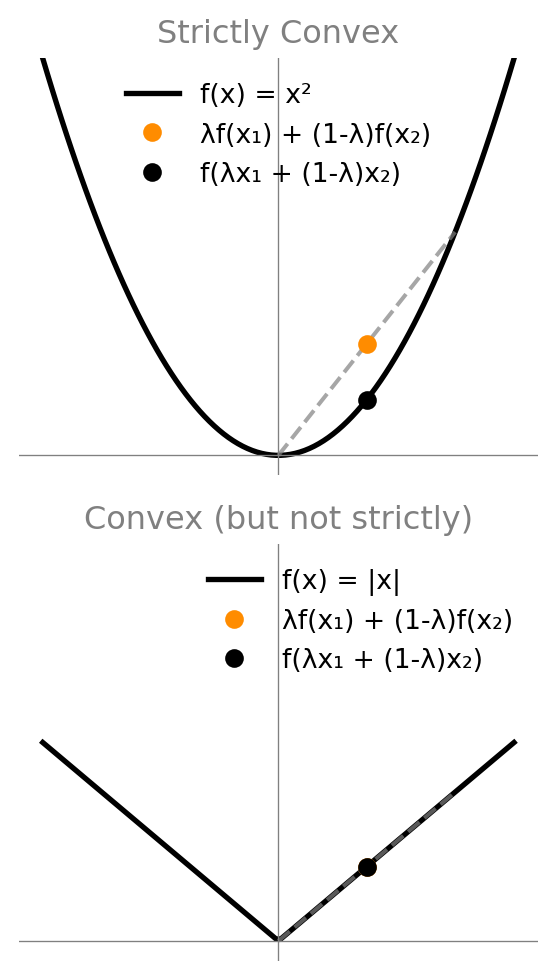
A function \(f\) is convex if for all \(x,y\) and \(\lambda \in [0,1]\): \[\lambda f(x) + (1-\lambda) f(y) \geq f(\lambda x + (1-\lambda) y).\]
Or, when \(f\) is twice differentiable: \[f''(x) \geq 0 \; \forall x.\]
Strictly convex if we have strict inequality: \(>\) instead of \(\geq\).
\(f\) is (strictly) concave if \(-f\) is (strictly) convex.
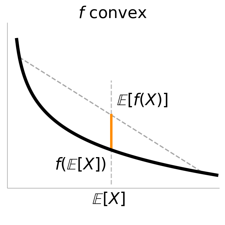
Jensen’s Inequality
Jensen’s Inequality
If \(f\) is convex, then for any random variable \(X\):
\[f(\implicitE{X}) \leq \implicitE{f(X)},\]
with equality if and only if one of the following holds:
- \(X\) is almost surely a constant.
- \(f\) is affine on the convex hull of the support of \(X\).
If \(f\) is strictly convex, then the inequality is strict unless \(X\) is (almost surely) a constant.
If \(f\) is concave, then the inequality is reversed.
Proof of Jensen’s Inequality
We start by showing:
Important
For \(f\) convex and \(\lambda_1, \lambda_2, \ldots, \lambda_n \geq 0\) with \(\sum_i \lambda_i = 1\):
\[f\left(\sum_i \lambda_i x_i\right) \leq \sum_i \lambda_i f(x_i).\]
We start with the definition of convexity: \[f(\lambda x + (1-\lambda) y) \leq \lambda f(x) + (1-\lambda) f(y).\]
Notice that this is equal to having \(\lambda_1, \lambda_2 \geq 0\) with \(\lambda_1 + \lambda_2 = 1\), such that:
\[f(\lambda_1 x_1 + \lambda_2 x_2) \leq \lambda_1 f(x_1) + \lambda_2 f(x_2).\]
We extend this to \(\lambda_1, \ldots, \lambda_n \geq 0\) with \(\sum_i \lambda_i = 1\) by iterating the convexity inequality:
\[ \begin{aligned} &f\left(\sum_i \lambda_i x_i\right) \\ &\quad \leq f\left((1-\lambda_n) \left(\sum_{i=1}^{n-1} \frac{\lambda_i}{(1-\lambda_n)} x_i\right) + \lambda_n x_n\right) \\ &\quad \leq (1-\lambda_n) f\left(\sum_{i=1}^{n-1} \frac{\lambda_i}{(1-\lambda_n)} x_i\right) + \lambda_n f(x_n) \\ &\quad = (1-\lambda_n) f\left(\sum_{i=1}^{n-1} \lambda_i' x_i\right) + \lambda_n f(x_n) \\ &\quad \leq (1-\lambda_n) \left(\cdots\right) + \lambda_n f(x_n) \\ &\quad \leq \sum_{i=1}^n \lambda_i f(x_i). \end{aligned} \]
with \(\lambda_i' \coloneqq \frac{\lambda_i}{1-\lambda_n} \geq 0\) for \(i=1,\ldots,n-1\) and \(\sum_{i=1}^{n-1} \lambda_i' = 1\).
Note that we have to drop any \(\lambda_i = 0\) to avoid division by zero, but we can obviously do that first w.l.o.g..
To make this formal, we can use induction to show, starting from \(n=2\) (already shown):
\(n = 2:\) \[f(\lambda_1 x_1 + \lambda_2 x_2) \leq \lambda_1 f(x_1) + \lambda_2 f(x_2).\]
\(n \to n+1\):
\[ \begin{aligned} f\left(\sum_{i=1}^{n+1} \lambda_i x_i\right) &\leq \sum_{i=1}^{n+1} \lambda_i f(x_i) \\ &\cdots \end{aligned} \]
[Left as exercise.] \(\square\)
Proof Sketch of Jensen’s Inequality
Now, we show the actual theorem:
Once we have this, we note that for any \(x_i \sim \pof{x}\), we have:
\[\frac{1}{n} \sum_i f(x_i) \overset{n \to \infty}{\longrightarrow} \E{\pof{x}}{f(x)},\]
by the law of large numbers.
Same for \(\frac{1}{n} \sum_i x_i \overset{n \to \infty}{\longrightarrow} \E{\pof{x}}{x}.\)
Then, by continuity of \(f\) (is it?), we have for \(\lambda_i = \frac{1}{n}\), \(x_i \sim \pof{x}\):
\[ \begin{aligned} f\left(\sum_{i=1}^n \lambda_i x_i\right) &\leq \sum_{i=1}^n \lambda_i f(x_i) \\ \overset{n \to \infty}{\longrightarrow} f\left(\E{\pof{x}}{x}\right) &\leq \E{\pof{x}}{f(x)}. \end{aligned} \]
\(\square\)
\(f\) convex \(\implies\) \(f\) continuous
…
See https://math.stackexchange.com/questions/258511/prove-that-every-convex-function-is-continuous
More on Convexity
More details can be found in the beautiful book by Boyd and Vandenberghe: https://web.stanford.edu/~boyd/cvxbook/bv_cvxbook.pdf
Convexity of \(\sicof{\cdot}\)
\(\forall \rho > 0: \frac{d^2}{d\rho^2} \sicof{\rho} = \frac{1}{\rho^2} > 0 \implies \sicof{\rho}\) strictly convex.
Entropy and Optimal Codes
Entropy
The entropy of a distribution is the average information content of a random variable:
\[\xHof{\pof{X}} \coloneqq \E{\pof{x}}{\sicof{\pof{x}}} = \E{\pof{x}}{-\ln \pof{x}}.\]
Example: Fair Coin
For a fair coin \(X\), we have \(\pof{\text{''Head''}} = \pof{\text{''Tail''}} = 0.5\) and:
\[\xHof{\pof{X}} = -0.5 \ln 0.5 - 0.5 \ln 0.5 = \ln 2 \text{ nats} = 1 \text{ bit}.\]
Example: Fully Biased Coin
For a fully biased coin \(X\) with \(\pof{\text{''Head''}} = 1\) and \(\pof{\text{''Tail''}} = 0\), we have:
\[\xHof{\pof{X}} = -1 \ln 1 - 0 \ln 0 = 0.\]
Deterministic Variable
For any deterministic variable \(X\) with \(\pof{x} = 1\) for some \(x\) and \(0\) otherwise, we have:
\[\xHof{\pof{X}} = -\ln 1 = 0.\]
Key Properties
- Conceptual Properties
- Measures uncertainty/randomness
- Higher entropy = greater uncertainty
- Mathematical Properties
- Non-negative: \(\xHof{\pof{X}} \geq 0\)
- Upper bounded: \(\xHof{\pof{X}} \leq \ln |\mathcal{X}|\) for discrete \(X\)
- Concavity: in \(\pof{x}\)
- Additivity: for independent variables: \(\xHof{\pof{X,Y}} = \xHof{\pof{X}} + \xHof{\pof{Y}}\) if \(X \indep Y\)
New Notation for \(\sicof{\cdot}\)
As notation of the information content, we will use:
\[\xHof{\pof{x}} \coloneqq \sicof{\pof{x}}.\]
When \(\pof{\cdot}\) is clear from context, we will simply write \(\Hof{\cdot}\).
So, \(\xHof{\pof{X}} = \E{\pof{x}}{\xHof{\pof{x}}}\) and \(\Hof{X} = \E{\pof{x}}{\Hof{x}}\).
Caution
The difference of \(\Hof{X}\) vs \(\Hof{x}\) is whether we take an expectation or not.
Non-Negativity of Discrete Entropy
The entropy of a discrete distribution is always non-negative:
Proof.
Individual Term Analysis: For each outcome \(x\), \(\pof{x} \in (0, 1]\).
Therefore, \(-\ln(\pof{x}) \geq 0\) because the natural logarithm of a probability \(\ln(\pof{x}) \leq 0\).
Summing Non-Negative Terms: Since each \(\pof{x} (-\ln \pof{x}) \geq 0\), their sum is also non-negative:
\[ \xHof{\pof{X}} = \sum_x \pof{x} (-\ln \pof{x}) \geq 0 \]
Equality Condition: Entropy \(\xHof{\pof{X}} = 0\) if and only if \(\pof{x} = 1\) for some \(x\) (i.e., the distribution is deterministic). \(\square\)
Source Coding Theorem
For any uniquely decodable code \(\mathcal{C}\) using an alphabet of size \(D\) with codeword lengths \(\ell_1, \ell_2, \ldots, \ell_m\) for \(x_1, x_2, \ldots, x_m\):
\[\xHof{\pof{X}} \le \sum_{i=1}^m \pof{x_i} \, \ell_i \text{ D-ary digits},\]
where \(\ln D \text{ nats}\) are \(1 \text{D-it (D-ary digit) }\) (like \(\ln 2 \text{ nats} = 1 \text{ bit}\)).
Proof
Define a pseudo-probability \(\qof{x_i}\) for each codeword:
\[ \begin{aligned} \qof{x_i} &\coloneqq \frac{\exp(-\ell_i \, \ln D)}{\sum_{i=1}^m \exp(-\ell_i \, \ln D)} \\ &= \frac{D^{-\ell_i}}{\sum_{i=1}^m D^{-\ell_i}}. \end{aligned}. \]
Note
Also known as the softmax function with temperature \(1 / \ln D\) (or more correctly, the softargmax function).
Then, we look at the following fraction on average and use Jensen’s inequality:
\[ \begin{aligned} \E{\pof{x}}{\sicof{\frac{\qof{x}}{\pof{x}}}} &= \E{\pof{x}}{-\ln \frac{\qof{x}}{\pof{x}}} \\ &\ge -\ln \E{\pof{x}}{\frac{\qof{x}}{\pof{x}}} \\ &= -\ln \sum_{i=1}^m \pof{x_i} \frac{\qof{x_i}}{\pof{x_i}} \\ &= -\ln \sum_{i=1}^m \qof{x_i} \\ &= -\ln 1 = 0. \end{aligned} \]
On the other hand, we have:
\[ \begin{aligned} &\E{\pof{x}}{\sicof{\frac{\qof{x}}{\pof{x}}}} \\ &\quad = \E{\pof{x}}{-\ln \frac{\qof{x}}{\pof{x}}} \\ &\quad = \E{\pof{x}}{-\ln \qof{x}} - \E{\pof{x}}{-\ln \pof{x}} \\ &\quad = \E{\pof{x}}{-\ln \qof{x}} - \xHof{\pof{X}}. \end{aligned} \]
Thus, overall:
\[\xHof{\pof{X}} \le \E{\pof{x}}{-\ln \qof{x}}.\]
Now, we substitute \(\qof{x}\) back:
\[ \begin{aligned} \xHof{\pof{X}} &\le \E{\pof{x}}{-\ln \frac{D^{-\ell(x)}}{\sum_{i=1}^m D^{-\ell_i}}} \\ &= \E{\pof{x}}{\ell(x) \, \ln D} + \ln \sum_{i=1}^m D^{-\ell_i}. \end{aligned} \]
From Kraft’s inequality, \(\sum_{i=1}^m D^{-\ell_i} \leq 1\), so the second term is non-positive because for \(x \le 1\), \(\ln x \leq 0\).
Thus, overall:
\[\xHof{\pof{X}} \le \ln D \, \E{\pof{x}}{\ell(x)}.\]\(\square\)
Note
For \(D=2\) with \(1 \text{ bit} = \ln 2 \text{ nats}\), we have:
\[\xHof{\pof{X}} \le \E{\pof{x}}{\ell(x)} \text{ bits}.\]
Tip
This shows that the entropy of a distribution is a lower bound on the expected codeword length of any prefix-free or uniquely decodable code.
Near-Optimal Code
Given \(\pof{x}\), we can construct a prefix-free code \(\mathcal{C}\) such that:
\[ \xHof{\pof{X}} \le \ln D \, \E{\pof{x}}{\ell(x)} \le \xHof{\pof{X}} + \ln D. \]
Note
Remember that \(\ln D \text{ nats}\) are \(1 \text{ D-it (D-ary digit) }\) (like \(\ln 2 \text{ nats} = 1 \text{ bit}\)). Thus:
\[ \xHof{\pof{X}} \le \E{\pof{x}}{\ell(x)} \text{ D-its} \le \xHof{\pof{X}} + 1 \text{ D-it}. \]
Given that we cannot send fractional messages easily—more on that later (maybe?)—this is as good as it gets essentially.
Proof
Recall that by Kraft’s inequality, if we have a sequence of code lengths \(\{\ell_i\}_{i=1}^m\) satisfying:
\[\sum_{i=1}^m D^{-\ell_i} \leq 1,\]
then there exists a prefix-free code with these lengths.
For a given distribution \(\pof{x}\), let’s choose code lengths:
\[\ell(x) \coloneqq \lceil -\log_D \pof{x} \rceil.\]
(\(\lceil y \rceil\) is the smallest integer greater than or equal to \(y\), i.e.
np.ceil).These lengths satisfy Kraft’s inequality:
\[\sum_{x} D^{-\ell(x)} \leq \sum_{x} D^{-(-\log_D \pof{x})} = \sum_{x} \pof{x} = 1,\]
where we used that \(\lceil y \rceil \geq y\) and thus \(D^{-\lceil y \rceil} \leq D^{-y}\).
For the upper bound on the expected code length:
\[ \begin{aligned} \E{\pof{x}}{\ell(x)} &= \E{\pof{x}}{\lceil -\log_D \pof{x} \rceil} \\ &\leq \E{\pof{x}}{-\log_D \pof{x} + 1} \\ &= -\frac{1}{\ln D}\E{\pof{x}}{\ln \pof{x}} + 1 \\ &= \frac{\xHof{\pof{X}}}{\ln D} + 1. \end{aligned} \]
Multiplying both sides by \(\ln D\) gives us:
\[\ln D \, \E{\pof{x}}{\ell(x)} \leq \xHof{\pof{X}} + \ln D. \] \(\square\)
Information Content & Optimal Code Length
The information content \(\Hof{x} = -\ln \pof{x}\) has a deep operational meaning: it specifies the optimal code length (in nats) for encoding an event \(x\) given its probability \(\pof{x}\). Let’s make this connection precise.
Our proof showed that the near-optimal code length is: \[\ell(x) = \lceil -\log_D \pof{x} \rceil\]
Expressing this in natural logarithms: \[\ell(x) \approx -\frac{\ln \pof{x}}{\ln D} = \frac{\Hof{x}}{\ln D}\]
For base \(e\) (nats): \[\ell(x) \approx \Hof{x}\]
Note
The ceiling function means we require fractionally more than \(\Hof{x}\) nats on average, bounded above by one extra nat as shown in the proof.
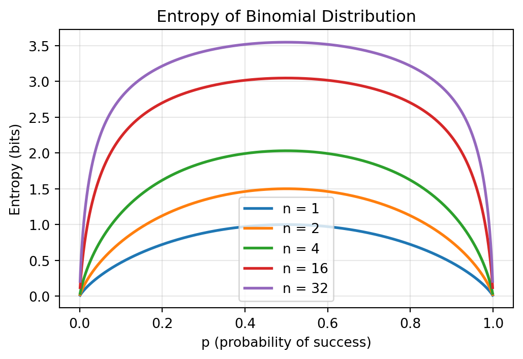
Example: Entropy of Discrete Distributions
- Maximum 1 bit at \(p=0.5\) (maximum uncertainty), and
- Minimum 0 as \(p\) approaches 0 or 1 (maximum certainty).
Fundamental principle: entropy is maximized when all outcomes are equally likely, and minimized when the distribution is concentrated on a single outcome.

- Maximum entropy at \(p=0.5\) for any fixed \(n\)
- Entropy increases with \(n\) due to more possible outcomes
Fundamental principle: entropy grows with the number of trials as the probability mass spreads across more possible outcomes, reflecting increased uncertainty in the total count.
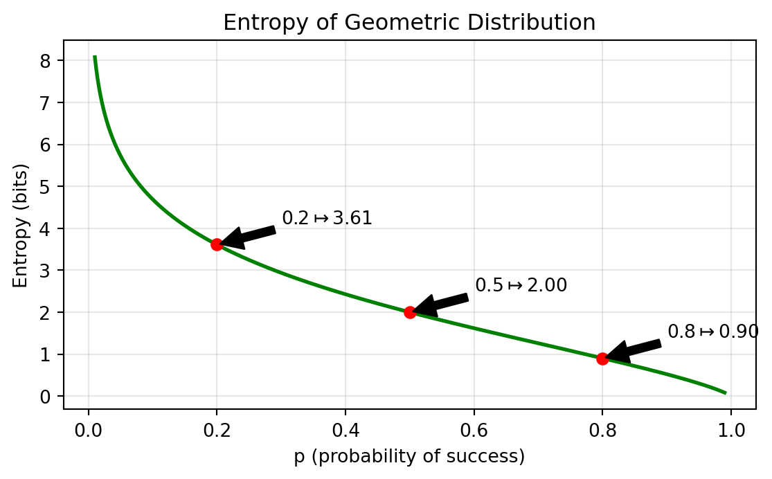
- Entropy \(\searrow\) as \(p\) \(\nearrow\) (shorter expected wait times)
- Minimum at \(p=1\) (immediate success)
- No upper bound as \(p \to 0\) (high uncertainty in wait time)
Fundamental principle: entropy grows with the uncertainty about the number of trials until success.
- Entropy increases with rate parameter λ
- Minimum entropy at \(λ = 0\) (certainty of zero events)
- No upper bound as \(λ → ∞\) (unbounded support)
Fundamental principle: entropy grows with the expected number of events, reflecting greater uncertainty in the final tally.

Key Empirical Observations
- Maximum entropy occurs when outcomes are equally likely
- Entropy increases with the spread of the distribution
- As distributions become more concentrated, entropy decreases
- The entropy of discrete distributions is always non-negative
Cross-Entropy & Kullback-Leibler
What happens if we use a near-optimal code for one distribution \(\qof{x}\) for symbols drawn from a different one \(\pof{x}\)?
How much worse than the best code for \(\pof{x}\) is this?
Comparing Codes
A code with codeword lengths \(\ell_{\opq}(x)\) for \(\qof{x}\) will use
\[ \E{\pof{x}}{\ell_{\opq}(x)} \text{ nats} \]
on average for symbols drawn from \(\pof{x}\).
This code is
\[ \E{\pof{x}}{\ell_{\opq}(x)} - \E{\pof{x}}{\ell_{\opp}} \text{ nats}\]
worse than a code \(\ell_\opp(x)\) for .
Comparing Near-Optimal Codes
\[ \begin{aligned} \xHof{\pof{X}} &\le \ln D \, \E{\pof{x}}{\ell^*(x)} \le \xHof{\pof{X}} + \ln D \\ \end{aligned} \]
Cross-Entropy
Given two distributions \(\opp\) and \(\opq\), the cross-entropy \[ \CrossEntropy{\pof{X}}{\qof{X}} \coloneqq \E{\pof{x}}{\Hof{\qof{x}}} = \E{\pof{x}}{-\ln \qof{x}}. \]
measures the average information content of samples drawn from \(\opp\) using \(\opq\).
Note
In some works, the cross-entropy is sometimes written as \(H(\pof{x}, \qof{x})\). We don’t do that.
Kullback-Leibler Divergence (🥬)
We can measure the divergence between using \(\qof{x}\) to encode samples from \(\pof{x}\) and \(\pof{x}\) itself, using the Kullback-Leibler divergence (KL divergence):
\[ \begin{aligned} \Kale{\pof{X}}{\qof{X}} &\coloneqq \CrossEntropy{\pof{x}}{\qof{x}} - \xHof{\pof{x}} \\ &= \E{\pof{x}}{-\ln \frac{\qof{x}}{\pof{x}}} \\ &= \E{\pof{x}}{\xHof{\frac{\qof{x}}{\pof{x}}}}. \end{aligned} \]
🥬 Non-Negativity?
\(\xHof{\pof{X}}\) gives us the optimal code length for encoding \(x\) under sampling from \(\pof{x}\).
The cross-entropy should always be worse than that:
Otherwise, we ought to use the code we can obtain from \(\xHof{\qof{X}}\) because it is better.
This is a contradiction to the lower-bound assumption.
Hence, the cross-entropy is always larger or equal the entropy:
\[ \begin{aligned} &\CrossEntropy{\pof{X}}{\qof{X}} \ge \xHof{\pof{X}} \\ \iff &\Kale{\pof{X}}{\qof{X}} \ge 0. \end{aligned} \] \(\square\)
🥬 Non-Negativity!
Let’s revisit our earlier proof on the entropy as a lower bound on the expected code length. The same idea yields:
\[ \begin{aligned} \Kale{\pof{X}}{\qof{X}} &= \E{\pof{x}}{\xHof{\frac{\qof{x}}{\pof{x}}}} \\ &\ge \xHof{\E{\pof{x}}{\frac{\qof{x}}{\pof{x}}}} \\ &= \xHof{\E{\qof{x}}{1}} \\ &= \xHof{1} = 0. \end{aligned} \] \(\square\)
Equality Case
Because \(\sicof{\rho} = -\ln \rho\) is strictly convex, the equality case \(\Kale{\pof{X}}{\qof{X}} = 0\) holds if and only if \(\frac{\qof{x}}{\pof{x}}\) is a constant function.
\(\frac{\qof{x}}{\pof{x}} = c \implies \qof{x} = c \pof{x}\).
Summing over all \(x\), we get \(1 = c\) because \(\opp\) and \(\opq\) are probability distributions.
Therefore, \(\qof{x} = \pof{x}\) for all \(x\).
Non-Negativity and Equality of 🥬 Divergence
For any distributions \(\pof{x}\) and \(\qof{x}\): \[\Kale{\pof{X}}{\qof{X}} \ge 0\]
Equality holds if and only if: \[\pof{x} = \qof{x} \text{ for (almost) all } x\]
This means the KL divergence acts as a measure of dissimilarity between distributions, though it is not symmetric and does not satisfy the triangle inequality.
🥬 Div & the Kraft Inequality
What is the difference the previous proof of the non-negativity of KL divergence and the proof on the lower bound of the entropy from earlier?
\(\qof{x}\) is already normalized!
Let \(Z \coloneqq \sum_x f(x)\) and \(\qof{x} \coloneqq \frac{f{x}}{Z}\).
\[ \begin{aligned} 0 &\le \E{\pof{x}}{\xHof{\frac{\qof{x}}{\pof{x}}}} \\ &\le \E{\pof{x}}{\xHof{\frac{f(x) / Z}{\pof{x}}}} \\ &= \E{\pof{x}}{\xHof{\frac{f(x)}{\pof{x}}}} + \ln Z \\ \iff \xHof{\pof{x}} &\le \E{\pof{x}}{\xHof{f(x)}} + \ln Z. \end{aligned} \]
If we set \(f(x) \coloneqq \exp(-\ell_\opq(x) \ln D) = D^{-\ell_\opq(x)}\), we recover the previous proof statement, and Kraft’s inequality is the constraint that \(Z \le 1\) for actual codes:
\[ \begin{aligned} \xHof{\pof{x}} &\le \E{\pof{x}}{\xHof{\qof{x}}} \\ &= \E{\pof{x}}{\xHof{f(x)}} + \ln Z \\ &\le \E{\pof{x}}{\xHof{D^{-\ell_{\opq}(x)}}} \\ &= \E{\pof{x}}{\ell_{\opq}(x)} \, \ln D \\ &= \E{\pof{x}}{\ell_{\opq}(x)} \text{ D-its}. \end{aligned} \]
Cross-Entropy Lower Bound
For any \(\pof{x}\),
\[ \begin{aligned} \xHof{\pof{X}} &\le \E{\pof{x}}{\xHof{\qof{x}}} \\ &\le \E{\pof{x}}{\ell_{\opq}(x)} \text{ D-its}. \end{aligned} \]
Multiple Variables
≙ Joint and Conditional (Cross-)Entropies ≙ Chain rule of KL divergence ≙ Chain rule of entropy
Joint & Conditional Info. Content
How?
Exactly as you would expect! We just plug more complex expressions into the definition \(-\ln \cdot\).
\[ \begin{aligned} \pof{x,y} &= \frac{\pof{x,y}}{\pof{x}} \pof{x} = \pof{x} \pof{y \given x} \end{aligned} \]
\[ \begin{aligned} \iff \log \pof{x,y} = \log \pof{x} + \log \pof{y \given x}. \end{aligned} \]
\[ \begin{aligned} \iff \Hof{x,y} &= \Hof{x} + \Hof{y \given x} \\ \iff \Hof{x \given y} &= \Hof{x,y} - \Hof{y}. \end{aligned} \]
Joint and Conditional Entropy
Entropy is an expectation over information content:
\[ \Hof{X} = \E{\pof{x}}{\Hof{x}} \]
\(\implies\) Same here.
\[ \Hof{X, Y} = \E{\pof{x, y}}{\Hof{x, y}} \]
\[ \Hof{X \given Y} = \E{\pof{x, y}}{\Hof{x \given y}} \]
Summary
For R.V.s \(X\), \(Y\):
Conditional Entropy
\[ \begin{aligned} \Hof{x \given y} &= \xHof{\pof{x \given y}}\\ \Hof{X \given Y} &= \E{\pof{x, y}}{\Hof{x \given y}} \end{aligned} \]
Chain Rule
\[ \begin{aligned} \Hof{x,y} &= \Hof{x} + \Hof{y \given x} \\ \Hof{X, Y} &= \Hof{X} + \Hof{Y \given X}. \end{aligned} \]
Conditional Joint Entropy
Write down what \(\Hof{x, y \given z}\) and \(\Hof{X, Y \given Z}\) are.
Note
\[ \begin{aligned} \Hof{x, y \given z} &= \sicof{\pof{x,y \given z}} \\ \Hof{X, Y \given Z} &= \E{\pof{x, y, z}}{\sicof{\pof{x,y \given z}}}. \end{aligned} \]
Expectation Decomposition
For random variables \(X\), \(Y\):
\[ \begin{aligned} \Hof{X \given Y} &= \E{\pof{x,y}}{\Hof{x \given y}} \\ &= \E{\pof{y}}{\E{\pof{x \given y}}{\Hof{x \given y}}} \\ &= \E{\pof{y}}{\Hof{X \given y}}. \end{aligned} \]
The intermediate equality follows from the tower rule (law of total expectation):
\[ \E{\pof{y}}{\E{\pof{x \given y}}{f(x,y)}} = \E{\pof{x,y}}{f(x,y)}. \]
Conditional Entropy \(\ge 0\)
If \(X\) is discrete, then:
\[ \Hof{X \given Y} = \E{\pof{y}}{\Hof{X \given y}} \ge 0. \]
because the entropy \(\Hof{X \given y}\) of the discrete random variable \(X \given y\) is non-negative for every \(y\).
Chain Rule of KL Divergence
The KL divergence between joint distributions decomposes into a sum of conditional KL divergences:
\[ \begin{aligned} &\Kale{\pof{X,Y}}{\qof{X,Y}} = \E{\pof{x,y}}{\xHof{\frac{\qof{x,y}}{\pof{x,y}}}} \\ &\quad = \E{\pof{x,y}}{\xHof{\frac{\qof{x}\qof{y \given x}}{\pof{x}\pof{y \given x}}}} \\ &\quad = \E{\pof{x}}{\xHof{\frac{\qof{x}}{\pof{x}}} + \E{\pof{x,y}}{\xHof{\frac{\qof{y \given x}}{\pof{y \given x}}}}} \\ &\quad = \Kale{\pof{X}}{\qof{X}} + \E{\pof{x}}{\Kale{\pof{Y \given x}}{\qof{Y \given x}}}. \end{aligned} \]
Shorter:
\[ \Kale{\pof{X,Y}}{\qof{X,Y}} = \Kale{\pof{X}}{\qof{X}} + \Kale{\pof{Y \given X}}{\qof{Y \given X}}. \]
Chain Rule of KL Divergence
The KL divergence between joint distributions equals the KL divergence between marginals plus the expected KL divergence between conditionals:
\[ \begin{aligned} \Kale{\pof{X,Y}}{\qof{X,Y}} &= \Kale{\pof{X}}{\qof{X}} \\ &\quad + \E{\pof{x}}{\Kale{\pof{Y \given x}}{\qof{Y \given x}}} \end{aligned} \]
This decomposition is particularly useful for:
- Analyzing sequential decision processes
- Understanding information flow in neural networks
- Deriving bounds on generalization error
Symmetry of Chain Rule
The chain rule in probability is symmetric:
\[ \pof{y} \pof{x \given y} = \pof{x,y} = \pof{x} \pof{y \given x}. \]
This leads to symmetric decompositions of the joint entropy (and information content):
\[ \Hof{Y} + \Hof{X \given Y} = \Hof{X,Y} = \Hof{X} + \Hof{Y \given X}. \]
Mutual Information
Rearranging these terms:
\[ \begin{aligned} &\Hof{X} - \Hof{X \given Y} = \Hof{Y} - \Hof{Y \given X} \\ &=\Hof{X} + \Hof{Y} - \Hof{X,Y} \end{aligned} \]
This quantity is called the mutual information between \(X\) and \(Y\). It measures the overlap in information between the two variables:
\[ \MIof{X ; Y} \coloneqq \Hof{X} + \Hof{Y} - \Hof{X,Y}. \]
M.I. as Reduction in Uncertainty
\[ \MIof{X ; Y} = \begin{cases} \begin{array}{c} \Hof{X} - \Hof{X \given Y} \\ ≙ \text{reduction in uncertainty about X} \end{array} \\[1em] \begin{array}{c} \Hof{Y} - \Hof{Y \given X} \\ ≙ \text{reduction in uncertainty about Y} \end{array} \\[1em] \begin{array}{c} \Hof{X} + \Hof{Y} - \Hof{X,Y} \\ ≙ \text{overlap in information} \end{array} \end{cases} \]
Properties of M.I.
- Conceptually:
- Measures the mutual dependence between R.V.s
- Can be expressed in multiple equivalent ways: reduction in uncertainty and overlap in information
- Mathematical properties:
- Symmetric: \(\MIof{X;Y} = \MIof{Y;X}\)
- Non-negative: \(\MIof{X;Y} \geq 0\)
- Independence: \(\MIof{X;Y} = 0\) if and only if \(X \indep Y\).
- Upper bound: \(\MIof{X;Y} \leq \min(\Hof{X}, \Hof{Y})\)
M.I. as KL Divergence
\[ \begin{aligned} \MIof{X ; Y} &= \Kale{\pof{X, Y}}{\pof{X}\pof{Y}} \\ &= \E{\pof{x,y}}{\xHof{\frac{\pof{x}\pof{y}}{\pof{x,y}}}} \\ &= \xHof{\pof{X}} + \xHof{\pof{Y}} - \xHof{\pof{X,Y}} \\ &= \Hof{X} + \Hof{Y} - \Hof{X,Y}. \end{aligned} \]
Mutual information measures the “distance” between the joint distribution and the product of marginals—exactly what we want for measuring dependence!
M.I. and Independence
\[ 0 = \MIof{X ; Y} = \Kale{\pof{X, Y}}{\pof{X}\pof{Y}} \]
iff \(\pof{x,y} = \pof{x} \, \pof{y}\) for all \(x,y\) from the equality case of KL divergence.
This is the definition of statistical independence.
\(\square\)
M.I. Non-Negativity
\[ \MIof{X ; Y} = \Kale{\pof{X, Y}}{\pof{X}\pof{Y}} \ge 0 \]
from the non-negativity of KL divergence.
\(\square\)
Conditioning Reduces Entropy
Conditioning Reduces Entropy
For any random variables \(X\) and \(Y\):
\[ \Hof{X \given Y} \le \Hof{X}, \]
with equality if and only if \(X \indep Y\).
Proof: Using the definition and non-negativity of mutual information:
\[ \begin{aligned} \Hof{X} &= \Hof{X \given Y} + \MIof{X;Y} \\ &\ge \Hof{X \given Y}. \end{aligned} \]
Intuition: Additional information can only reduce our uncertainty.
Equality Case: When \(X\) and \(Y\) are independent, knowing \(Y\) provides no information about \(X\).
M.I. Upper Bound
\(\MIof{X ; Y} = \Hof{X} - \Hof{X \given Y} \le \Hof{X}.\)
Same for \(\Hof{Y}\).
Thus, \(\MIof{X ; Y} \le \min(\Hof{X}, \Hof{Y})\).
\(\square\)
Convexity and Concavity
From Conditioning to Concavity
Let’s show that entropy is concave in \(\pof{x}\). That is, for any distributions \(\pof{x}\) and \(\qof{x}\):
\[ \begin{aligned} &\xHof{\lambda \pof{X} + (1-\lambda) \qof{X}} \\ &\quad \ge \lambda \xHof{\pof{X}} + (1-\lambda) \xHof{\qof{X}}. \end{aligned} \]
Consider a binary random variable \(Z\) with \(\pof{Z=1} = \lambda.\)
Let \(X\) be distributed according to \(\pof{x}\) when \(Z=1\) and \(\qof{x}\) when \(Z=0\).
Then: \[ \pof{x \given z} = \begin{cases} \pof{x} & \text{if } z = 1 \\ \qof{x} & \text{if } z = 0 \end{cases} \]
And the marginal distribution of \(X\) is: \[ \pof{x} = \lambda \pof{x} + (1-\lambda) \qof{x}. \]
\(\square\)
Formal Statement
The entropy \(\xHof{\pof{X}}\) is concave in \(\pof{x}\).
Proof:
From conditioning reduces entropy: \[\Hof{X} \ge \Hof{X \given Z}\]
The LHS is: \[\Hof{X} = \xHof{\lambda \pof{X} + (1-\lambda) \qof{X}}\]
The RHS is: \[ \begin{aligned} \Hof{X \given Z} &= \lambda \Hof{X \given Z=1} + (1-\lambda) \Hof{X \given Z=0} \\ &= \lambda \xHof{\pof{X}} + (1-\lambda) \xHof{\qof{X}} \end{aligned} \]
Therefore: \[ \begin{aligned} &\xHof{\lambda \pof{X} + (1-\lambda) \qof{X}} \\ &\quad \ge \lambda \xHof{\pof{X}} + (1-\lambda) \xHof{\qof{X}} \end{aligned} \] \(\square\)
Max. and Min. Discrete Entropy
The entropy \(\xHof{\pof{X}}\) is concave in \(\pof{x}\).
We already know that entropy is non-negative and is 0 for deterministic distributions.
This means uncertainty is maximized by spreading out probability mass (i.e. through mixing).
For discrete variables with \(n\) states, the maximum entropy is achieved by the uniform distribution:
\[ \xHof{\pof{X}} \le \ln n. \]
Proof:
\[ \begin{aligned} \Kale{\pof{X}}{\mathrm{Uniform}(X)} &= \ln n - \xHof{\pof{X}} \\ &\ge 0 \\ \iff \ln n &\ge \xHof{\pof{X}}. \end{aligned} \]
Convexity of KL Divergence
The KL divergence \(\Kale{\pof{X}}{\qof{X}}\) is convex in \(\pof{x}\) and convex in \(\qof{x}\):
\[ \begin{aligned} &\lambda \Kale{\pcof{1}{X}}{\qcof{1}{X}} + (1-\lambda) \Kale{\pcof{2}{X}}{\qcof{2}{X}} \\ &\quad \ge \Kale{\lambda \pcof{1}{X} + (1-\lambda) \pcof{2}{X}}{\lambda \qcof{1}{X} + (1-\lambda) \qcof{2}{X}}, \end{aligned} \]
for \(\lambda \in [0,1]\), \(\pcof{1}{x}\), \(\pcof{2}{x}\), \(\qcof{1}{x}\), and \(\qcof{2}{x}\) any distributions.
Proof.
For any \(\lambda \in [0,1]\), let \(Z \sim \mathrm{Bernoulli}(\lambda)\) with \(\pof{z}\) and \(\qof{z}\) both following this distribution.
Set up \(\pof{x \given z = 0} = \pcof{2}{x}\) and \(\pof{x \given z = 1} = \pcof{1}{x}\) and likewise for \(\opq\), \(\opq_1\), \(\opq_2\).
Then, we can express the mixture as:
\[ \begin{aligned} &\lambda \Kale{\pcof{1}{X}}{\qcof{1}{X}} + (1-\lambda) \Kale{\pcof{2}{X}}{\qcof{2}{X}} \\ &\quad = \E{\pof{z}}{\Kale{\pof{X \given z}}{\qof{X \given z}}} + 0. \end{aligned} \]
\(\pof{z} = \qof{z}\), \(\Kale{\pof{Z}}{\qof{Z}} = 0\) and with the chain rule of KL divergence:
\[ \begin{aligned} &= \E{\pof{z}}{\Kale{\pof{X \given z}}{\qof{X \given z}}} + \Kale{\pof{Z}}{\qof{Z}} \\ &= \Kale{\pof{X, Z}}{\qof{X, Z}} \\ &= \E{\pof{x}}{\Kale{\pof{Z \given x}}{\qof{Z \given x}}} + \Kale{\pof{X}}{\qof{X}} \\ &\ge \Kale{\pof{X}}{\qof{X}} = \\ &= \Kale{\lambda \pcof{1}{X} + (1-\lambda) \pcof{2}{X}}{\lambda \qcof{1}{X} + (1-\lambda) \qcof{2}{X}}, \end{aligned} \]
as \(\E{\pof{x}}{\Kale{\pof{Z \given x}}{\qof{Z \given x}}} \ge 0\) by non-negativity of the KL divergence.
Therefore:
\[ \begin{aligned} &\lambda \Kale{\pcof{1}{X}}{\qcof{1}{X}} + (1-\lambda) \Kale{\pcof{2}{X}}{\qcof{2}{X}} \\ &\quad \ge \Kale{\lambda \pcof{1}{X} + (1-\lambda) \pcof{2}{X}}{\lambda \qcof{1}{X} + (1-\lambda) \qcof{2}{X}}, \end{aligned} \]
and the KL divergence is convex in \(\pof{x}\) and \(\qof{x}\). \(\square\)
Generalizing Mutual Information
From Two to Many Variables
Mutual information for two variables measures their dependency:
\[\MIof{X;Y} = \Hof{X} + \Hof{Y} - \Hof{X,Y}\]
How do we extend this to more variables?
For three variables, we can define the interaction information:
\[\MIof{X;Y;Z} = \MIof{X;Y} - \MIof{X;Y \given Z}\]
Key Insight
This measures how much the mutual information between X and Y changes when we condition on Z.
Alternative Forms
The interaction information has several equivalent forms:
\[ \begin{aligned} \MIof{X;Y;Z} &= \MIof{X;Y} - \MIof{X;Y \given Z} \\ &= \MIof{X;Z} - \MIof{X;Z \given Y} \\ &= \MIof{Y;Z} - \MIof{Y;Z \given X} \end{aligned} \]
Symmetry
All these forms are equivalent due to the symmetry of information measures!
Inclusion-Exclusion Form
We can also write interaction information as an alternating sum:
\[ \begin{aligned} \MIof{X;Y;Z} = &\Hof{X,Y,Z} \\ &-\Hof{X,Y} - \Hof{X,Z} - \Hof{Y,Z} \\ &+\Hof{X} + \Hof{Y} + \Hof{Z} \end{aligned} \]
The XOR Example
Consider three binary variables \(X\), \(Y\), \(Z\) where:
- \(X\) and \(Y\) are independent fair coin flips
- \(Z = X \oplus Y\) (exclusive OR)
| X | Y | Z | |
|---|---|---|---|
| 00 | 0 | 0 | 0 |
| 01 | 0 | 1 | 1 |
| 10 | 1 | 0 | 1 |
| 11 | 1 | 1 | 0 |
Properties of XOR
- X and Y are independent: \(\MIof{X;Y} = 0\)
- Z is determined by X,Y: \(\Hof{Z|X,Y} = 0\)
- But individually: \(\MIof{X;Z} = \MIof{Y;Z} = 0\)
Key Result
The interaction information is negative: \[\MIof{X;Y;Z} = -1 \text{ bit}\]
Computing XOR’s Interaction Information
Let’s verify \(\MIof{X;Y;Z} = -1\) bit:
First, \(\MIof{X;Y} = 0\) (independence)
Then, \(\MIof{X;Y|Z}\): \[ \begin{aligned} \MIof{X;Y|Z} &= \Hof{X|Z} - \Hof{X|Y,Z} \\ &= 1 - 0 = 1 \text{ bit} \end{aligned} \]
Therefore: \[\MIof{X;Y;Z} = \MIof{X;Y} - \MIof{X;Y|Z} = 0 - 1 = -1 \text{ bit}\]
Interpreting Negative Interaction Information
When \(\MIof{X;Y;Z} < 0\):
- Knowledge of Z increases dependency between X and Y
- Variables exhibit “synergy” - they work together
- Common in:
- Error correction codes
- Neural networks
- Cryptographic systems
Summary
Interaction information generalizes mutual information to multiple variables
Unlike two-variable MI, it can be negative
Negative values indicate:
- Synergistic relationships
- Increased dependencies under conditioning
- Complex variable interactions
XOR provides the canonical example
Beyond Three Variables
For n variables \(X_1, \ldots, X_n\), we can define higher-order interaction information recursively:
\[\MIof{X_1;\ldots;X_n} = \MIof{X_1;\ldots;X_{n-1}} - \MIof{X_1;\ldots;X_{n-1} \given X_n}\]
Properties
Inclusion-Exclusion Form: Can be written as sum of entropies:
\[\MIof{X_1;\ldots;X_n} = \sum_{S \subseteq \{1,\ldots,n\}} (-1)^{|S|+1} \Hof{X_S}\]
This generalizes the three-variable case we saw earlier.
Symmetry: Order of random variables doesn’t matter
Sign Interpretation: Can be:
- Positive (redundant information)
- Negative (synergistic information)
- Zero (independent random variables?)
Self-Information = Entropy
For any random variable \(X\):
\[ \begin{aligned} \MIof{X;X} &= \Hof{X} - \Hof{X \given X} \\ &= \Hof{X} - 0 \\ &= \Hof{X}. \end{aligned} \]
\(\Hof{X \given X} = 0\) because \(X \given X\) is deterministic!
Tip
The entropy \(\Hof{X}\) is the mutual information of a random variable with itself 🤯
Example: Four Variables
The inclusion-exclusion form involves:
- 4 single entropies/self-informations
- 6 (pairwise) mutual informations
- 4 triple mutual informations
- 1 quadruple mutual information
Total: 15 information quantities!
Key Insight
The inclusion-exclusion principle provides a systematic way to compute higher-order interactions, though the number of terms grows exponentially with n. This is why most applications focus on lower-order interactions (n ≤ 3).
“Duality”
For 4 variables, we also have 15 information quantities using joint entropies:
- Entropy Basis:
- 4 single entropies: \(\Hof{X}\), \(\Hof{Y}\), \(\Hof{Z}\), \(\Hof{W}\)
- 6 joint entropies of pairs: \(\Hof{X,Y}\), \(\Hof{X,Z}\), …
- 4 joint entropies of triples: \(\Hof{X,Y,Z}\), …
- 1 joint entropy of all: \(\Hof{X,Y,Z,W}\)
- Mutual Information Basis: See previous slide.
Key Insight
The inclusion-exclusion formulas are “change-of-basis” transformations. Each basis offers a different but equivalent way to describe information relationships.
Information Diagrams
Information diagrams (I-diagrams) provide a simple visualization of information-theoretic quantities and their relationships, similar to Venn diagrams for sets.
Example

Key Idea
Areas in I-diagrams represent entropy quantities, with overlaps showing mutual information.
Basic Properties
- Areas = Information
- Individual regions represent entropy (or information content)
- Overlaps show mutual information
- Total area equals joint entropy
- Signed Quantities
- Unlike Venn diagrams, some regions can be negative
- Particularly important for >2 variables
- Geometric Relations
- \(\Hof{X,Y} = \Hof{X} + \Hof{Y} - \MIof{X;Y}\)
- \(\Hof{X \given Y} = \Hof{X} - \MIof{X;Y}\)
Two-Variable I-Diagram
Three-Variable I-Diagram

Attention!
Triple overlaps can be negative:
\[\MIof{X;Y;Z} \overset{?}{<} 0.\]
Important Differences from Venn Diagrams
Venn Diagrams
- Set relationships
- Always non-negative areas
- Direct visual inequalities
- Simple interpretation
I-Diagrams
- Information quantities
- Can have negative regions
- Complex relationships
- Careful interpretation needed
I-Diagrams: Theory
Based on Yeung (1991):
Yeung, Raymond W. “A new outlook on Shannon’s information measures.” IEEE transactions on information theory 37.3 (1991): 466-474.
A Signed Measure
Information diagrams provide a principled framework for reasoning about information quantities.
Yeung (1991) showed we can define a signed measure μ* mapping information to set operations:
\[ \begin{aligned} \IMof{A} &= \Hof{A} \\ \IMof{\cup_i A_i} &= \Hof{A_1, \ldots, A_n} \\ \IMof{\cup_i A_i - \cup_i B_i} &= \Hof{A_1, \ldots, A_n \given B_1, \ldots, B_n} \\ \IMof{\cap_i A_i} &= \MIof{A_1;\ldots; A_n} \\ \IMof{\cap_i A_i - \cup_i B_i} &= \MIof{A_1;\ldots; A_n \given B_1,\dots,B_n} \end{aligned} \]
Measures: A Quick Review
A function \(\mu\) mapping sets to numbers is a measure if:
Non-negativity: \(\mu(A) \geq 0\)
Null empty set: \(\mu(\emptyset) = 0\)
Countable additivity: For disjoint sets \(\{A_i\}\):
\[ \mu(\cup_i A_i) = \sum_i \mu(A_i) \]
Examples
- Lebesgue measure (length, area, volume)
- Probability measure (total mass = 1)
- Counting measure (counts elements)
Signed Measures
A signed measure relaxes non-negativity:
Extended real-valued: \(\mu(A) \in [-\infty, \infty]\)
Null empty set: \(\mu(\emptyset) = 0\)
Countable additivity: For disjoint \(\{A_i\}\):
\[ \mu(\cup_i A_i) = \sum_i \mu(A_i) \]
At most one infinity: Not both \(+\infty\) and \(-\infty\)
Key Insight
Yeung’s I-measure μ* is a signed measure, allowing for: - Negative mutual information terms - Preservation of additivity properties - Rigorous treatment of information quantities
I-Measure as Signed Measure
Yeung’s I-measure μ* maps information to set operations:
\[ \begin{aligned} \IMof{A} &= \Hof{A} \\ \IMof{\cup_i A_i} &= \Hof{A_1, \ldots, A_n} \\ \IMof{\cap_i A_i} &= \MIof{A_1;\ldots; A_n} \end{aligned} \]
Important!
- Satisfies additivity but allows negative values
- Makes I-diagrams mathematically rigorous
- Bridges set theory and information theory
Beyond Venn Diagrams
Key Difference
- Mutual information terms with >2 variables can be negative
- Cannot always read inequalities directly
- Set intuitions may mislead
Atomic Quantities
An atomic quantity quantity involves all variables in the system under consideration. For a system of n variables, atomic quantities cannot be decomposed into simpler terms involving fewer variables.
Example: Three-Variable Case
For variables X, Y, Z, the atomic quantities are:
- Conditional Entropies: \(\Hof{X\given Y,Z}\), \(\Hof{Y\given X,Z}\), \(\Hof{Z\given X,Y}\).
- Conditional Mutual Information: \(\MIof{X;Y|Z}\), \(\MIof{X;Z|Y}\), \(\MIof{Y;Z|X}\).
- Triple Mutual Information: \(\MIof{X;Y;Z}\)
Key Property
When atomic quantities equal zero, they can be safely eliminated from I-diagrams. For example, if \(\MIof{X;Y \given Z} = 0\), we can remove that region without affecting other relationships.
Zero MI ≠ Empty Intersection
Consider \(\MIof{X;Y} = 0\):
- Does NOT imply X and Y regions are disjoint
- Could have Z where \(\MIof{X;Y;Z} < 0\)
- Then: \[\MIof{X;Y} = \MIof{X;Y;Z} + \MIof{X;Y \given Z} = 0\] but \(X \cap Y \neq \emptyset\)
Common Mistake
Don’t assume zero mutual information means regions can be separated in the diagram!
Example: Markov Chain
For a Markov chain \(X_1 \to X_2 \to X_3\):

Key Property
In a Markov chain, non-adjacent variables are fully “explained” by any intermediate variable: \[ \MIof{X_1 ; X_3 \given X_2} = 0. \]
Applications of I-Diagrams
- Visualizing Dependencies
- Conditional independence
- Information bottlenecks
- Markov properties
- Understanding Inequalities
- Data processing inequality
- Information can’t increase
- Conditioning reduces entropy
- Teaching Tool
- Intuitive understanding
- Quick sanity checks
- Relationship visualization
Common Pitfalls
Be Careful!
- Not All Inequalities Visible
- Some relationships need algebra
- Visual intuition can mislead
- Negative Regions Possible
- Especially with >2 variables
- Can’t always trust area comparisons
- Zero MI ≠ Empty Intersection
- Independence more subtle than disjointness
- Need careful interpretation
Summary
I-diagrams provide visual intuition for information relationships
Key differences from Venn diagrams:
- Can have negative regions
- More complex interpretations
- Not all relationships visible
Useful for:
- Understanding dependencies
- Visualizing inequalities
- Teaching information theory
But require careful interpretation!
Recap
Core Concepts Mastered
- Information Content & Entropy
- Quantified uncertainty with \(\sicof{\pof{x}} = -\ln \pof{x}\)
- Understood entropy as average information
- Proved key properties (non-negativity, concavity)
- Optimal Coding
- Connected information content to code lengths
- Proved source coding theorem
- Constructed near-optimal codes
- Multiple Variables
- Extended concepts to joint/conditional entropy
- Mastered chain rules and decompositions
- Explored mutual information
- Visual Reasoning
- Learned I-diagram framework
- Distinguished from Venn diagrams
- Avoided common pitfalls
Key Skills
- Rigorous mathematical reasoning
- Information-theoretic intuition
- Visual thinking with I-diagrams
Next Steps
- Apply to machine learning (next lecture)
- Explore continuous variables
Bibliography
- Cover, T.M. and Thomas, J.A.. Elements of information theory. Wiley-Interscience, 2006(Cover and Thomas 2006)
- Yeung, Raymond W. Information theory and network coding. Springer Science & Business Media, 2008. (Yeung 2008)
- MacKay, David J.C.. Information theory, inference and learning algorithms. Cambridge University Press, 2003. (MacKay 2003)
- Chapters §1.2 and §2 of my thesis (Kirsch 2024)
References
Cover, Thomas M., and Joy A. Thomas. 2006. Elements of Information Theory (Wiley Series in Telecommunications and Signal Processing). USA: Wiley-Interscience.
Huffman, David A. 1952. “A Method for the Construction of Minimum-Redundancy Codes.” Proceedings of the IRE 40 (9): 1098–1101.
Kirsch, Andreas. 2024. “Advancing Deep Active Learning & Data Subset Selection: Unifying Principles with Information-Theory Intuitions.” arXiv Preprint arXiv:2401.04305.
Lang, Leon, Pierre Baudot, Rick Quax, and Patrick Forré. 2022. “Information Decomposition Diagrams Applied Beyond Shannon Entropy: A Generalization of Hu’s Theorem.” arXiv Preprint abs/2202.09393. https://arxiv.org/abs/2202.09393.
MacKay, David JC. 2003. Information Theory, Inference and Learning Algorithms. Cambridge university press.
McGill, William J. 1954. “Multivariate Information Transmission.” Transactions of the IRE Professional Group on Information Theory 4: 93–111. https://doi.org/10.1109/TIT.1954.1057469.
Shannon, Claude Elwood. 1948. “A Mathematical Theory of Communication.” The Bell System Technical Journal 27 (3): 379–423.
Yeung, Raymond W. 1991. “A New Outlook on Shannon’s Information Measures.” IEEE Transactions on Information Theory 37 (3): 466–74.
———. 2008. Information Theory and Network Coding. Springer Science & Business Media.