import matplotlib.pyplot as plt
from sklearn.datasets import make_classification
from sklearn.ensemble import RandomForestClassifier
import numpy as np
np.random.seed(42)
# Generate synthetic dataset
X, y = make_classification(n_samples=1000, n_features=20,
n_informative=15, n_redundant=5,
random_state=42)
# Split into labeled and unlabeled pools
sampled_idx = np.random.choice(len(X), 100, replace=False)
X_labeled = X[sampled_idx]
y_labeled = y[sampled_idx]
# Main active learning loop
random_query_loss = {}
model = RandomForestClassifier()
for i in range(1, len(sampled_idx) + 1):
model.fit(X_labeled[:i], y_labeled[:i])
loss = model.score(X, y)
random_query_loss[i] = loss
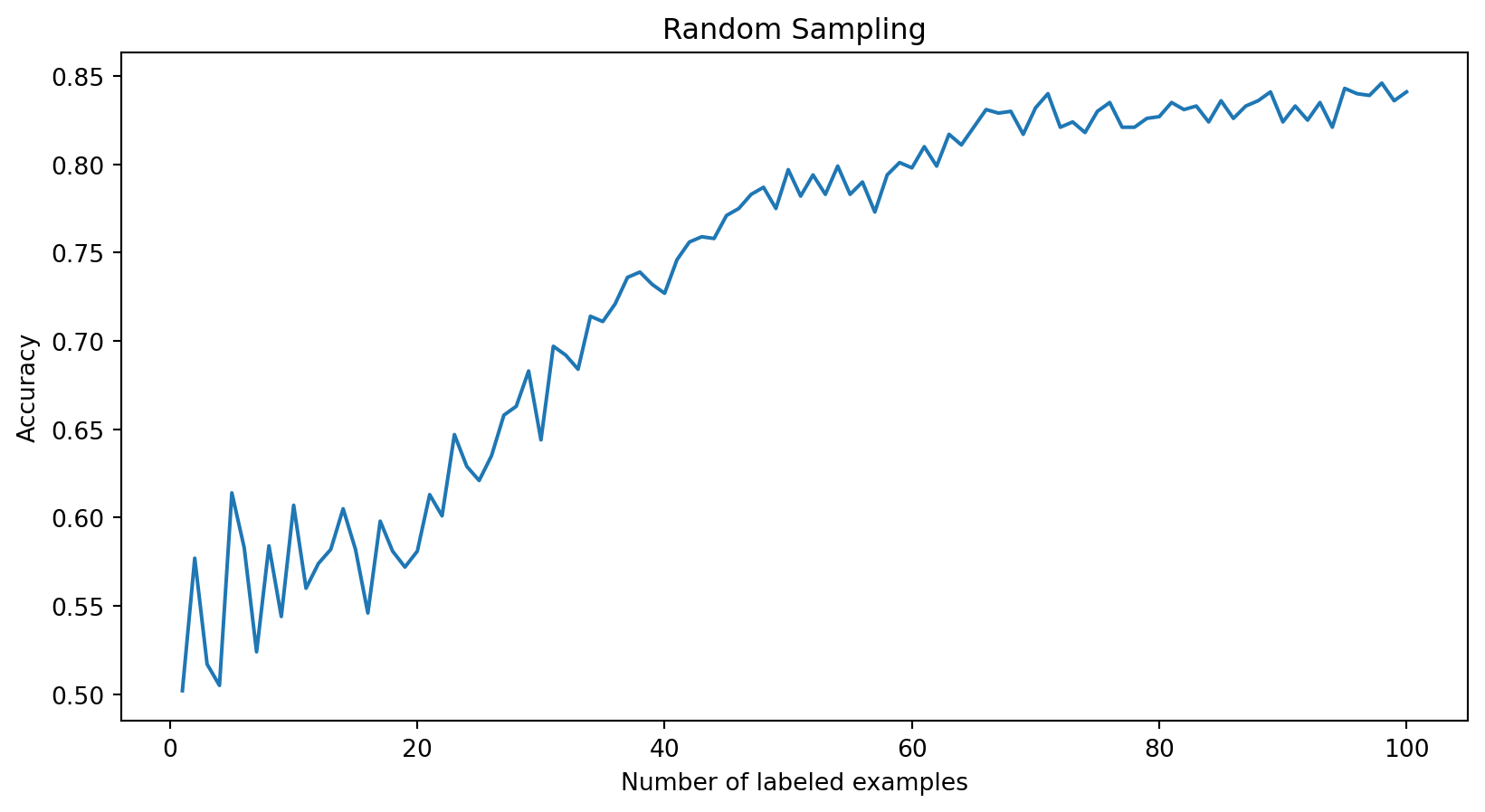
plt.plot(list(random_query_loss.keys()), list(random_query_loss.values()))
plt.xlabel("Number of labeled examples")
plt.ylabel("Accuracy")
plt.title("Random Sampling")
plt.show()Active Learning
More Data-Efficient Machine Learning
Andreas Kirsch
Why AL Matters
Imagine training a model for a self-driving car. Each labeled image costs $50 and you need millions. How do you choose which images to label?
Key Insight
Not all training examples contribute equally to model learning. Active learning helps identify and prioritize the most valuable data.
Today’s Promise
By the end of this lecture, you’ll understand:
- Why active learning can cut labeling costs by 90%
- Three practical strategies to implement it
- How to choose the right approach for your problem
The Power of Asking Questions
Think of active learning like a curious student who asks strategic questions:
- Instead of reading the whole textbook
- They identify key concepts they don’t understand
- And ask the teacher focused questions about those
This is exactly what active learning does.
In “Active Learning”
Active learning is a machine learning meta-algorithm that strategically selects its own training data:
- Instead of passively accepting a pre-defined training set,
- The learner actively queries an oracle (typically a human expert) for labels
- Thus for the data to add to the training set.
Meta-Algorithms
A meta-algorithm is an algorithm that operates on or controls another algorithm.
Think of it like a teacher (oracle) guiding a student (* model) by choosing what examples to study and in what order (meta-algorithm*).
Non-AL Meta-Algorithm Example
- Algorithm: Computes gradients and updates parameters
- Meta-Algorithm: Learning rate scheduler that:
- Monitors training progress
- Adjusts the learning rate dynamically
- Decides when to reduce/increase step sizes
The scheduler (meta) controls how the optimizer (base) learns, just like active learning controls what the model learns.
In the context of active learning:
- The base algorithm is the machine learning model (e.g., neural network, SVM)
- The meta-algorithm is the active learning strategy that:
- Controls what data the base model sees
- Decides when and what to query
- Manages the learning process
Traditional ML vs Active Learning
Normal ML
- Uses fixed training set
- Sees all labels upfront
- No data selection strategy
Pool-Based Active Learning
- Grows dataset incrementally
- Strategically selects examples
- Learns from feedback loop
# Given: unlabeled_pool = [x1, ..., xn]
model = initialize_model()
labeled_dataset = []
oracle = HumanExpert()
# or other labeling source

# Iteratively grow training set
while len(labeled_dataset) < budget:
    # Score all unlabeled examples
    scores = acquisition_function(model, unlabeled_pool)

    # Select most promising example(s)
    x_next = unlabeled_pool[argmax(scores)]

    # Query oracle for label
    y_next = oracle.label(x_next)

    # Add to training set and update model
    labeled_dataset.append((x_next, y_next))
    model = initialize_model()
    for epoch in range(num_epochs):
        for x, y in labeled_dataset:
            model.train_step(x, y)

    # Remove queried example from pool
    unlabeled_pool.remove(x_next)
Let’s Code: A Simple Example
Using a random query strategy (as baseline)
Let’s Code: A Simple Example
The Many Faces of Active Learning
AL Applications: Why?
We can identify three main real-world scenarios where active learning can be applied:
- Speech recognition: Annotating 1 hour of audio takes 10 hours of expert time
- Medical imaging: Radiologists’ time costs $200+/hour
- Drug discovery: Each experiment costs (hundreds of) thousands of dollars
- Protein folding: Crystallography is expensive and time-consuming (“one PhD for one protein”)
- AI Safety: Labeling model outputs for alignment, safety, and bias detection
- Human Preference Data: Collecting feedback on response quality and naturalness (RLHF)
- Instruction-Output Pairs: Creating high-quality examples of desired model behavior
- Expert Domain Validation: Verifying factual accuracy and specialized knowledge
- Training large models requires massive compute resources
- Active learning can help by selecting the most informative training examples
- Instead of training on all data, we can:
- Sample a subset of training data strategically
- Focus compute on the most valuable examples
- Reduce training costs while maintaining performance
AL Scenarios: Where?
- Most common scenario in practice
- Large pool of unlabeled data available upfront
- Query strategy evaluates and ranks all candidates
- Selects most informative examples to label
- Examples: Image classification, text categorization
labeled_data = [(x1,y1), ..., (xk,yk)]
n_initial = len(labeled_data)
# Given: large unlabeled pool
unlabeled_pool = [x{k+1}, ..., xn]

while len(labeled_data) < n_initial + budget:
    # Train model
    model = train_model(labeled_data)

    # Score ALL examples at once
    scores = acquisition_fn(model, unlabeled_pool)

    # Select best example(s)
    best_idx = argmax(scores)
    x_next = unlabeled_pool[best_idx]

    # Query and update
    y = oracle.label(x_next)
    labeled_data.append((x_next, y))
unlabeled_pool.remove(x_next)- Data arrives sequentially, one at a time
- Must decide immediately: query or discard
- Cannot compare against future examples
- Often uses uncertainty threshold
- Examples: Social media monitoring, sensor networks
labeled_data = [(x1,y1), ..., (xk,yk)]
n_initial = len(labeled_data)

# Process data stream one at a time
threshold = 0.7  # uncertainty threshold

for x in data_stream:
    # Train model
    model = train_model(labeled_data)

    # Immediate decision required
    uncertainty = compute_uncertainty(model, x)

    if uncertainty > threshold:
        y = oracle.label(x)
        labeled_data.append((x, y))
        if len(labeled_data) >= n_initial + budget:
            break
    else:
continue # ignore example- Generates artificial examples to query
- Model can query any point in input space
- Challenging for human oracles (may be unrealistic)
- More common in experimental design
- Examples: Drug discovery, robotics control
labeled_data = [(x1,y1), ..., (xk,yk)]
n_initial = len(labeled_data)

while len(labeled_data) < n_initial + budget:
    # Generate candidate points
    candidates = []
    for _ in range(n_candidates):
        x = generate_synthetic_example()
        candidates.append(x)

    # Select most promising point
    x_next = optimize_acquisition(candidates)

    # Query oracle with synthetic point
    y = oracle.label(x_next)
    labeled_data.append((x_next, y))
Problem Settings
- Goal: Minimize labeling costs while maximizing model performance
- Setting: Access to unlabeled data and labeling oracle
- Process:
- Model selects informative examples
- Oracle provides labels
- Model updates with new labeled data
- Key Challenge: Selecting examples that will improve model most
- Cost: Primarily labeling effort (time/money)
- Goal: Optimize training compute by selecting most valuable examples
- Setting: Working with already labeled dataset
- Process:
- Score training examples by potential value
- Select subset for current training iteration
- Update scoring based on model state
- Key Challenge: Balancing exploration vs exploitation during training
- Cost: Primarily computation time
Curriculum Learning
Curriculum Learning is a special case of active sampling where:
- Examples are ordered by difficulty
- Training progresses from easy to hard
- Difficulty measure is usually fixed and pre-defined
Key Difference
Active sampling is online—it adapts dynamically to the model’s current state—while curriculum learning is offline—follows a pre-defined ordering of examples.
- Goal: Efficiently evaluate model performance with minimal test queries
- Setting: Limited budget for test-time inference
- Process:
- Strategically select test examples
- Estimate overall performance from subset
- Adapt selection based on uncertainty
- Key Challenge: Getting reliable performance estimates from few samples
- Cost: Test-time computation or API calls
Query Strategies: How?
- Query strategies select valuable examples for labeling, using
- Acquisition functions, which score unlabeled examples
Note
We aim to estimate how informative a sample would be if we could train on it, allowing us to prioritize the most valuable examples for model improvement.
Query Strategies: Uncertainty Sampling
The simplest and most intuitive approach: query the examples where the model is least confident.
Three main variants:
Selects examples where the model’s highest predicted probability is lowest.
This focuses on examples where the model struggles to make a clear prediction.
Considers the difference between the two highest predicted probabilities.
Small margins indicate the model is uncertain between two competing classes.
Uses information-theoretic entropy to measure uncertainty across all classes.
High entropy indicates uniform predictions across classes, suggesting high uncertainty.
Query Strategies: Query-by-Committee
Maintains an ensemble and queries disagreement.
High disagreement indicates high informativeness, so we query where the committee is divided.
def query_by_committee(models, unlabeled_pool):
    # Get predictions from all models
    predictions = [model.predict(unlabeled_pool) for model in models]

    # Compute disagreement (vote entropy)
    disagreement = compute_vote_entropy(predictions)

    return unlabeled_pool[np.argmax(disagreement)]
Theoretical Insight
QBC actively reduces the version space - the set of hypotheses consistent with the labeled data.
Advanced Query Strategies
Select examples that would cause the largest change in model parameters:
\[x^* = \arg\max_x \mathbb{E}_{y \sim p(y|x)} \left[\|\theta_{t \mid {y, x}} - \theta_t\|\right],\]
where \(\theta_{t \mid {y, x}}\) are the model parameters after also training on \(x\) labeled with \(y\).
Choose examples that minimize expected future error:
\[x^* = \arg\min_x \mathbb{E}_{y \sim p(y|x)} [\sum_{x' \in \mathcal{X}_\text{pool}} \mathbb{E}_{y' \sim p(y'|x')} \mathcal{L}(\theta_{t \mid y, x}; y', x') ].\]
Important
Why does this not contain the current loss?
Practical Considerations
Real-world Challenges (and Approaches):
- Batch querying for parallel labeling
- Noisy oracles and disagreement
- Variable labeling costs
- When to stop querying?
Let’s Code: A Simple Example
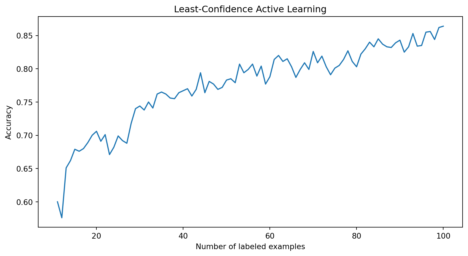
Using uncertainty sampling via confidence scores
import random

def least_confidence_score(model, unlabeled_pool):
    probs = model.predict_proba(unlabeled_pool)
    confidence = np.max(probs, axis=1)
    return -confidence

labeled_indices = list(sampled_idx[:10])
pool_indices = list(set(range(len(X))) - set(labeled_indices))

confidence_loss = {}
for _ in range(len(labeled_indices),len(random_query_loss)):
    model = RandomForestClassifier()
    model.fit(X[labeled_indices], y[labeled_indices])

    scores = least_confidence_score(model, X[pool_indices])
    pool_index = np.argmax(scores)
    labeled_indices.append(pool_indices[pool_index])
    del pool_indices[pool_index]

    loss = model.score(X, y)
    confidence_loss[len(labeled_indices)] = loss

plt.plot(list(confidence_loss.keys()), list(confidence_loss.values()))
plt.xlabel("Number of labeled examples")
plt.ylabel("Accuracy")
plt.title("Least-Confidence Active Learning")
plt.show()
Let’s Code: A Simple Example
Our First Results
plt.plot(random_query_loss.keys(), random_query_loss.values(), label="Random")
plt.plot(confidence_loss.keys(), confidence_loss.values(), label="Confidence")
plt.legend(); plt.xlabel("Number of labeled examples"); plt.ylabel("Accuracy")
plt.title("Least-Confidence Active Learning vs Random Sampling"); plt.show()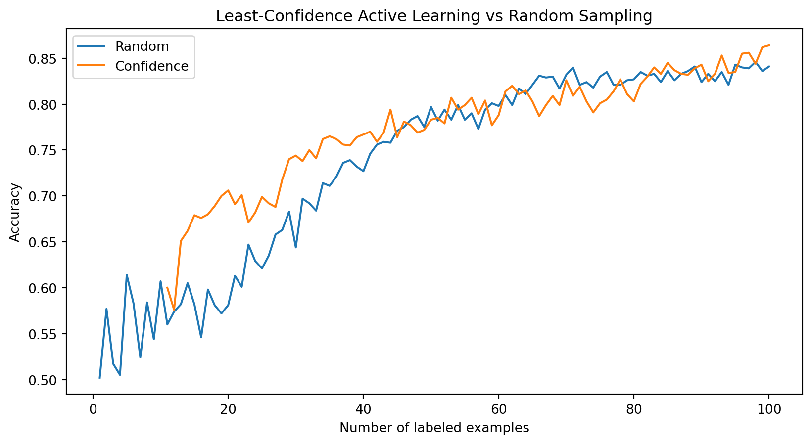
Preview
In the next lectures, we’ll dive deeper into:
- Information-theoretic approaches to active learning
- Bayesian active learning
- Deep (Bayesian) active learning
Summary
So what we have learned today:
- Active learning reduces labeling costs through strategic sampling
- Simple strategies like least-confidence sampling can already work better than random sampling
- Practical constraints in real applications
- Different AL scenarios and settings
Further Reading
Settles, Burr. 2009. “Active Learning Literature Survey.”